The highs and lows of Digital Elevation Model (DEM) error - developing a spatially distributed DEM error model.

Bruce H. Carlisle
School of Earth and Environmental Sciences, University of Greenwich, Chatham Maritime, Kent, ME4 4TB, UK
E-mail: b.h.carlisle@gre.ac.uk

Abstract

Despite the last decade’s increasing concern for understanding and working with the uncertainty within DEMs, knowledge about DEM error is still at a basic stage and incorporation of this knowledge into DEM-based modelling applications has only developed to a limited extent. This research addresses the limitations of using a single Root Mean Square Error value to portray the uncertainty associated with a DEM by developing a technique for creating a spatially distributed DEM error model – an error surface.

The technique is based on the hypothesis that the distribution and scale of errors within a DEM are at least partly related to characteristics of the terrain. The technique involves the collection of high accuracy elevation measurements to compute DEM error, the generation of a set of terrain parameters to characterise the terrain and developing regression models to define the relationship between DEM error and terrain character. The regression models form the basis for creating a RMSE surface to portray DEM error. These error surfaces provide more detailed information about DEM error than a single global estimate of RMSE and an initial assessment of these surfaces indicates they are of sufficient quality for use in stochastic simulations of the impact of DEM error on spatial modelling applications. Error surfaces also have the potential to open the door to a more deterministic approach towards incorporation of uncertainty into spatial modelling by means of probabilistic modelling techniques.

1. Introduction

Spatial modelling often achieves only limited success due to the quality of source data. It has been known for some time that digital elevation data, and other spatial data sets, are subject to inherent errors (Clark, 1993; Fisher, 1994; Goodchild & Han, 1995). The past decade has seen a series of authors, for example Weibel & Brändli (1995), urging DEM users to appraise the quality of their elevation data and the derived DEMs. Having made a DEM quality assessment the user needs to consider the influence of DEM quality on derived products and models, as stated by Miller and Morrice (1996) in particular reference to hydrological models. Despite the last decade’s increasing concern for understanding and working with the uncertainty within DEMs, knowledge about DEM error is still at a basic stage and incorporation of this knowledge into DEM-based modelling applications has only developed to a limited extent.

Assessment of DEM quality is commonly restricted to reporting a Root Mean Square Error (RMSE) value. For example, in the UK, the Ordnance Survey’s digital contour data has a quoted accuracy of +/- 1.0m to 1.8m RMSE (REF). The United States Geological Survey (USGS) describes the accuracy of its 7.5 minute DEMs with one RMSE value for each quadrangle or tile. This RMSE value is based on the difference between DEM elevation and the elevation of test points measured by field survey or aerotriangulation, or from a spot height or point on a contour line from an existing source map (USGS, 1997). The RMSE for each quadrangle is calculated from 28 test points. Such error estimates have three limitations:

the error estimate often describes error in the source elevation data, e.g. contour lines and spot heights, rather than the derived DEM;
the error estimate often does not relate to true elevation, but the elevation recorded in another data source;
a single nationwide figure in the case of the Ordnance Survey or a quadrangle-wide figure in the case of the USGS is a global estimate, which does not reflect the spatially varying nature of DEM error. It is known, when deriving a DEM from stereo pairs of aerial photographs, that errors are likely to be larger on shaded (steep and northerly facing) slopes and on smooth, featureless terrain. This knowledge of the variation in error is not communicated by the single RMSE value.

The single global error estimates of DEM error have been used to visualise DEM quality by showing “epsilon bands” around contour lines and catchment boundaries, e.g. Chrisman (1983), and by using stochastic techniques, such as Monte Carlo simulation to derive a sample of potentially valid model outputs reflecting the influence of DEM uncertainty on the modelling process, (Miller and Morrice, 1996; Fisher, 1994; Monckton, 1994). A spatially distributed model of DEM error would provide a more detailed and reliable basis for stochastic simulations than a single RMSE value, but could also open the door to a more deterministic approach towards incorporating DEM error knowledge into spatial modelling. This approach could involve probabilistic techniques, based on the probability that a cell was higher than its neighbours.

This paper describes the development of a spatially distributed model of DEM error (an error surface), which could be used in probabilistic modelling techniques. The technique is based on the hypothesis that the errors in a DEM are at least partly related to the nature of the terrain. Identifying the relationship between error and terrain parameters, such as slope, curvature or relative relief, allows one to create an error surface.

2. Objectives

Quantify the error present in DEMs;
Derive a large set of terrain parameters from the DEMs;
Investigate and define the relationship between elevation error and different terrain parameters;
Use the defined error / terrain relationship to generate error surfaces.

3. Methods

3.1 Study Area and Data

Spatial modelling involving DEM data sets are undertaken in a wide range of application areas and for all types of environment. The broader focus of the research described here is on hydrological modelling in mountain environments. However, this research is of relevance both to other types of terrain or environments and to other application areas.

The primary study area for this research is a 2km x 1.3km region of Snowdonia, North Wales, UK. Ordnance Survey 1:10,000 scale Landform Profile digital contours with a vertical interval of 10m have been used to generate DEMs with a 1m horizontal resolution. The key stages of the Snowdonia research have been reapplied to a 23.5km x 18.1km region of Mestersvig, northeast Greenland. The Greenland study area is used to validate that the findings in Snowdonia are applicable to other mountain regions and to different scales of source data and DEMs. Manual digitising of 50m contours on 1:15,000 scale Mylar contour maps derived from aerial photography has been used to generate DEMs with a 10m horizontal resolution.

GPS survey techniques have been used to measure true elevation to an accuracy of +/- 0.9m RMSE. 106 points have been surveyed in the Snowdonia study area. 103 points have been surveyed in the Greenland study area.

3.2 DEM Generation

26 DEMs have been generated for the Snowdonia study area, using various interpolation techniques, for ongoing research into the nature an extent of DEM error. For the purposes of deriving a distributed error surface, three of these 26 DEMs have been used. These are:

SpTen12 - the most accurate of the 26 DEMs, produced using ArcView's spline with tension interpolator and a 12 point search radius;
IDW512 - the most accurate inverse distance weighting DEM, produced using ArcView's inverse distance weighting interpolator with a weight of 5 and a 12 point search radius;
IDW16 - the least accurate inverse distance weighting DEM, produced using ArcView's inverse distance weighting interpolator with a weight of 1 and a 6 point search radius.

3.3 Terrain Parameters

For each of the three DEMs figures the following 11 terrain parameters have been derived and extracted at each GPS survey point:

1. Elevation.
2. Slope angle (or gradient).
3. Plan curvature.
4. Profile curvature.
5. Relative relief:
        The range of elevation values of all grid cells within a 10-cell radius of the grid cell concerned.
6. Texture:
        A measure of the ruggedness of the terrain calculated as the range of slope values of all grid cells
        within a 10-cell radius of the grid cell concerned.
7. Mean extremity:
        The elevation of a grid cell minus the mean elevation of all grid cells within a 10-cell radius of that
        grid cell. Indicates the elevation of the grid cell relative to its neighbours.
8. Minimum extremity:
        The elevation of a grid cell minus the lowest elevation of all grid cells within a 10-cell radius of that
        grid cell. A value of near zero would indicate that that grid cell is in a pit.
9. Maximum extremity:
        The elevation of a grid cell minus the highest elevation of all grid cells within a 10-cell radius of that
        grid cell. A value of near zero would indicate that that grid cell is on a peak.
10. Standard deviation:
        The standard deviation of elevation values of all grid cells within a 10-cell radius of the grid cell
        concerned.
11. Point distance:
        The distance between a grid cell and the nearest of the contour vertices from which the DEM was
        interpolated.

3.4 Correlations

Coefficients for the correlation between each terrain parameter and DEM error have been calculated to give an initial indication of the presence of a relationship. Two measures of elevation error have been used: the original signed elevation errors; and the difference between a survey point’s error and the mean error for that DEM - termed the mean error difference here (see Equation 3.5.1).

Equation 3.5.1

3.5 Further Terrain Parameters

Due to a high degree of short range variation observed in most of the terrain parameters described in section 3.3, mean smoothing filters were applied to parameters 2 to 4 in the above list to derive additional terrain parameters. Circular filter windows of 5, 10 and 20 cell radii were applied. Second, terrain parameters 5 to 10 in the above list were recalculated using 5 and 20 cell radii. Third, each of the resulting set of terrain parameters was squared and cubed in order to allow polynomial (quadratic and cubic) coeficients in the regression modelling described below. This led to a total of 96 terrain parameters for each DEM.

3.6 Further Correlations

The correlations of section 3.5 were repeated for all 96 terrain parameters.

3.7 Defining the Terrain Parameter / DEM Error Relationship

Multiple linear regression has been used to define the relationship between the terrain parameter values and DEM error at the 100+ GPS survey points. Although linear regression techniques have been used, the inclusion of squared and cubed terrain parameters emulates polynomial regression. First, regressions between all 96 terrain parameters and the DEM errors have been assessed. Second, a stepwise selection procedure has been used to develop an optimum regression model using just 20 of the 20 terrain parameters.

3.8 Error Surfaces

Having derived regression equations modelling the relationship between DEM error and the terrain parameters at the 100+ GPS survey points, the next step is to apply the equation to the whole study area to produce an error surface. This has been achieved by applying map algebra to raster images representing each of the variables in the respective regression equations. To allow the quality of the error surfaces to be assessed, minimum, maximum, mean and standard deviation values for each error surface have been calculated.

4. Results

4.1 Correlations

Table 4.1.1 summarises the correlations between the DEM errors and the initial set of 11 terrain parameters for the Snowdon study area.

Table 4.1.1. Summary of Snowdon correlations between terrain parameters and DEM error.
Table 3.5.1

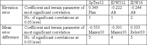
The correlations indicate, first, that the relationship is stronger for mean error difference than signed error and, second, that the relationship is strongest for the spline with tension DEM. However, although 5 out of 11 correlation coefficients for the mean error difference of SpTen12 are significant, the correlations are only weak or moderately strong.

4.2 Further Correlations

Table 4.2.1 summarises the correlations between the DEM errors and all 96 terrain parameters for the Snowdon study area.

Table 4.2.1. Summary of further correlations between terrain parameters and DEM error.
Table 3.7.1

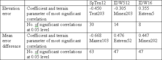
Table 4.2.1 illustrates again that the SpTen12 DEM gives the strongest correlations and the greatest number of significant correlations. Also there are a far greater number of significant correlations and stronger correlations between the terrain parameters and the mean error difference. Although stronger correlations have been found than for the initial 11 terrain parameters, they are still only moderately strong. However, there is clear evidence of a relationship between DEM error and the characteristics of the terrain, which could be defined through regression modelling.

4.3 Defining the Terrain Parameter / DEM Error Relationship

The results of multiple linear regression using signed error and mean error difference as the dependant variable and all 96 terrain parameters as the independant variables are shown in Table 4.3.1.

Table 4.3.1. Coefficients for multiple linear regression using all 96 terrain parameters.
Table 3.8.1

The R² value is an estimate of the proportion of values that will be correctly predicted by applying the calculated regression equation to unknown values of Y, which in this case is elevation error at unsampled locations. The more variables that are used in the multiple regression the more likely it is that the independent variables (the terrain parameters) can be made to fit the dependent variable (elevation error) within the scope of the sample. When fitting 96 independent variables to 100+ observations it is highly likely that the R² value is overly optimistic. The adjusted R² value takes account of the number of variables used and gives a more realistic indication of how well the calculated regression equation will predict unknown elevation errors. It is this adjusted R² value that should be used to judge the effectiveness of the regressions performed.

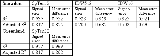
The adjusted R² values for Snowdon’s SpTen12 DEM indicate that attempting to predict the elevation error throughout the DEM is potentially viable. This is also true of Greenland’s SpTen12 DEM. The values for the other two DEMs are not so promising.

In order to predict elevation error for an entire DEM, a raster image is required for each of the terrain parameters used in the multiple regression modelling. Creation of 96 images and the subsequent map algebra required to replicate the regression equation as an error surface image is not practical. It is also inefficient as many of the terrain parameters have little influence on the regression model. So the next step in modelling elevation error is to find the best regression equation using only a limited number of terrain parameters. This has been achieved using a stepwise regression procedure, adding or removing one variable to the regression at each step. Figure 3.8.1 plots the number of variables used against the corresponding adjusted R² values for Snowdon’s SpTen12 DEM. The graph shows that there is little increment in the adjusted R² values beyond 20 variables. Generating an error surface from 20 images is computationally feasible. Therefore regression equations, and subsequently the error surfaces, have been generated from the best 20 variables.

Figure 4.3.1. Graph of Adjusted R² plotted against number of variables.
Figure 3.8.1

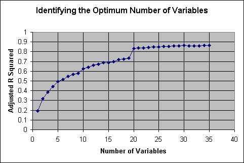
Table 4.3.2 gives the regression coefficients for the 20 variables selected by stepwise regression modelling. As with the multiple regression using all 96 terrain parameters, the terrain parameters derived from SpTen12 have markedly stronger goodness-of-fit with the error values. Further work concentrates solely on the SpTen12 DEMs.

Table 4.3.2. Coefficients for stepwise regression using 20 variables.
Table 3.8.2

4.4 Error Surfaces

Table 4.4.1 gives summary statistics for both the error surfaces and the GPS survey points in terms of minimum, maximum, mean and standard deviation values.

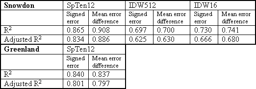
Table 4.4.1. Error surfaces’ summary statistics.
Table 3.9.1

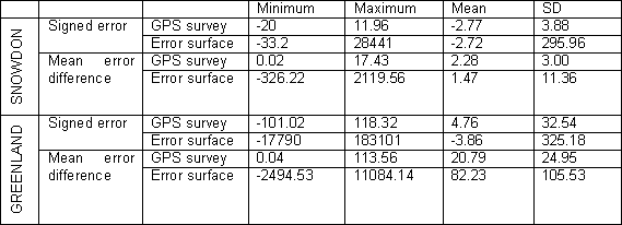
The error surfaces’ summary statistics would seem to indicate that the regression equations perform poorly when extrapolated to a whole study area. Greenland’s signed error surface has a maximum error more than 20 times as high as Mount Everest! Both the mean error difference surfaces have negative values, which are invalid. All of the four error surfaces are characterised by a high degree of short-range variability.

To reduce the short range variability of the error surfaces and suppress the extreme values a smoothing mean filter has been applied, using a circular window of 20-cell radius. Additionally, the intention of this research is not to produce a cell by cell exact estimate of elevation error, but to produce a spatially distributed model of RMSE, which improves on a single global RMSE value. So RMSE has been calculated for each cell and its 20-cell radius circular neighbourhood. Summary statistics for the resulting RMSE surfaces are given in Table 4.4.2.

Table 4.4.2. RMSE surfaces’ summary statistics.
Table 3.9.2

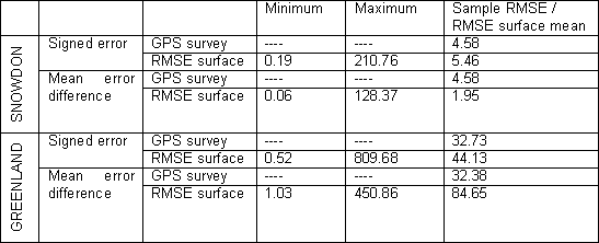
The process of filtering and creating an RMSE surface removes the most extreme cell values, although high maximum values remain. However, in Snowdon the proportion of cells with an RMSE greater than 25m is 1.93% for the RMSE surface derived from the signed error values and 1.15% for the RMSE surface derived from mean error difference values. For Greenland the proportion of cells with an RMSE greater than 250m is 0.22% for the RMSE surface derived from the signed error values and 2.08% for the RMSE surface derived from mean error difference values. Histograms for the RMSE surface values are given in Figure 4.4.1 to Figure 4.4.4.

Figure 4.4.1. Histogram of RMSE values derived from signed error for Snowdon.
Figure 3.9.1

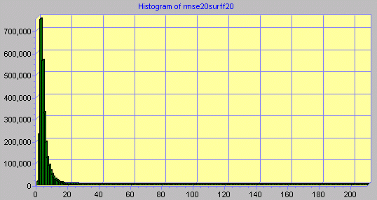
Figure 4.4.2. Histogram of RMSE values derived from mean error difference for Snowdon.
Figure 3.9.2

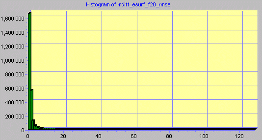
Figure 4.4.3. Histogram of RMSE values derived from signed error for Greenland.
Figure 3.9.3

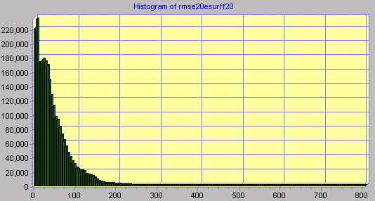
Figure 4.4.4. Histogram of RMSE values derived from mean error difference for Greenland.
Figure 3.9.4

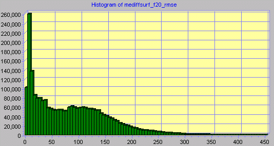
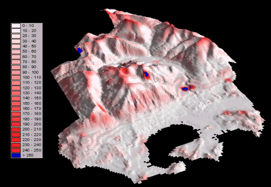
Figure 4.4.5 and Figure 4.4.6 show orthographic perspective views of Snowdon’s RMSE surface derived from mean error difference and Greenland’s RMSE surface derived from signed error draped over the corresponding DEMs.

Figure 4.4.5. Orthographic perspective view of Snowdon’s RMSE surface derived from mean error difference draped over the SpTen12 DEM.
Figure 3.9.5

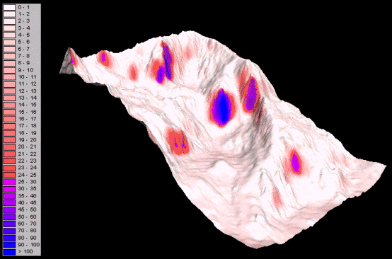
Figure 4.4.6. Orthographic perspective view of Greenland’s RMSE surface derived from mean error difference draped over the SpTen12 DEM.
Figure 3.9.6

5. Discussion

The correlation coefficients in Table 4.2.1 show that characteristics of the terrain, as defined by terrain parameters, do influence the scale and distribution of DEM error. The stepwise regression modelling results indicate that this influence can be defined by a regression equation. However, there are differences in results for the different DEMs. The relationship between DEM error and terrain characteristics has been better defined for the DEM created with spline interpolation than for those created using inverse distance weighted algorithms. Spline interpolation produces smooth rounded surfaces and consequently more gradually changing values for the derived terrain parameters. The nature of the inverse distance weighting algorithms produces DEMs with artefacts including flat topped peaks and "puddles" (circular areas of near constant elevation) around the contour vertices. It seems that these artefacts obscure the underlying error / terrain relationship.

There are also differences in terms of the specific terrain parameters used in the stepwise regression modelling. Table 5.0.1 shows the number of occurrences of each type of terrain parameter used as variables in the regression equations for the SpTen12 DEMs.

Table 5.0.1 Number of occurrences of terrain parameters in stepwise regressions.
Table 3.8.3

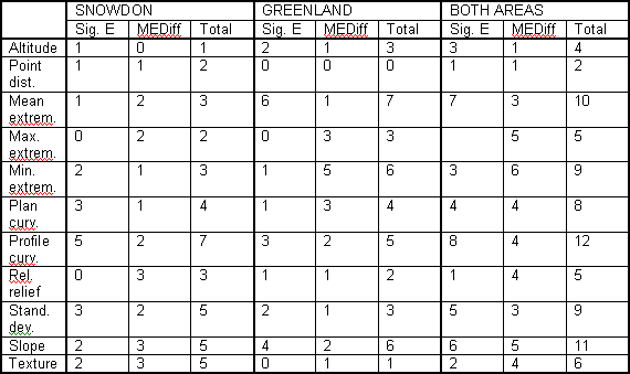
The terrain parameters used in the regression equations vary between Snowdon and Greenland and between signed error and mean error difference. Point distance is used least frequently and only in the Snowdon equations. Profile curvature, slope and mean extremity are used most frequently. However, it is evident that the most “useful” types of terrain parameter vary depending both on the type of error and the location being modelled. No universal regression equation is apparent. It would seem that the factors influencing the distribution and scale of DEM errors are specific both to the nature of the terrain being modelled and to the way in which the original elevation data have been captured.

Table 4.4.1 indicates that the initial error surfaces derived from the regression equations are of limited quality. It is to be expected that the error surfaces have problems. First, the regression equations are only based on a limited number of GPS survey points. Although these points represent a variety of terrain characteristics, only accessible locations can be surveyed. So the steepest and most rugged terrain is not represented. Consequently, the extreme and invalid error values are found in the steepest and most rugged areas. Second, the adjusted R² values of about 0.8 to 0.85 indicate a reasonable, but not great, goodness-of-fit. So some poor predictions of error and extreme values within the error surfaces are to be expected. Table 4.4.2 shows that mean filtering and calculation of RMSE values suppresses the initial error surface problems. However, the resulting RMSE surfaces are now only approximations of the variation in error over the study areas, rather than the exact predictions of the initial error surfaces. But an approximation of the error is realistically the best that can be expected for three reasons. First, DEM error has only been measured at a limited number of survey points. Although the survey points were selected so as to give the best possible representation of the variety of terrain characteristics present in each study area, the most inaccessible areas could not be included. Second, the terrain parameters are derived from DEMs containing error and will be subject to error themselves. Therefore, it is not possible to define an exact relationship between DEM and terrain parameters. Third, while a large number of terrain parameters have been derived from the DEMs, these parameters may not be the optimum for characterising the terrain and its relationship with DEM error. In particular, the use of 5, 10 and 20 cell radii may not be the best. It may be beneficial to employ a more computer-intensive approach, in which terrain parameters are calculated over a greater number of radii.

The quality of the RMSE surfaces in terms of the summary statistics in Table 4.4.2 and the histograms in Figure 4.4.1 to Figure 4.4.4 reflects the adjusted R² values of the corresponding regression equations. For Snowdon, the regression with mean error difference has the higher adjusted R² value (0.886 compared to 0.834 for signed error) and the resulting RMSE surface has lower minimum, maximum and mean and a lower percentage of cells greater than 25m. For Greenland, the regression with signed error has the higher adjusted R² value (0.801 compared to 0.797 for minimum error difference) and the resulting RMSE surface has lower minimum and mean values and lower percentage of cells greater than 250m.

The orthographic views of Figure 4.4.5 and Figure 4.4.6 indicate that the RMSE surfaces appear “sensible”. Although the distribution of error values differs between Snowdon and Greenland, in both locations the relationship between DEM error and terrain characteristics can be discerned. In Snowdon the highest values coincide with the steepest slopes, which are near-vertical rock outcrops or cliff faces. In the case of Greenland, the highest values tend to lie along the ridges. It is probable that the differences in distribution are due to both differences in the terrain characteristics of the two areas and the differences in the scales of source data and DEMs.

6.0 Conclusions

This research has shown that there is a relationship between terrain characteristics and a DEM’s elevation error. This relationship is strongest for DEMs produced using a spline interpolator. The technique presented - GPS surveying of true elevation, deriving terrain parameters and regression modelling - allows a RMSE surface to be created. Such RMSE surfaces seem to provide a reasonable approximation of the actual spatial variation in DEM error over an area. The technique is based on terrain parameters derived from an “error-full” DEM. Consequently, the terrain parameters, the regression modelling and the resultant RMSE surface will be prone to some degree of error. Nonetheless, the spatially distributed RMSE surface provides a greater amount of information about a DEM’s error than the single global RMSE figures available to date.

The set of terrain parameters, which provides the optimum regression with elevation error, is location specific. In this study 20 terrain parameters have been chosen from a total of 96 based on terrain characteristics within 5m, 10m and 20m radii of a target cell. Terrain parameters based on other radii may be more effective. A more truly GeoComputation-style approach may be beneficial, in which terrain parameters for a whole range of radii are computed and assessed.

When applied to stochastic simulations, RMSE surfaces have the potential to give a better account of the influence of DEM error on modelling outcomes than use of a single RMSE value. Work is continuing to develop probabilistic hydrological models, which work with a DEM and an accompanying RMSE surface. The outcomes of this further work will demonstrate the usefulness of the RMSE surfaces developed here, and the additional knowledge of DEM error that they provide.

References

Chrisman, N.R., 1983. Epsilon filtering: a technique for automated scale changing. Proceedings of 1983 ACSM Annual Meeting, 322-331.

Clark, K.J., 1993. Data constraints on GIS application development. In: Kovar, K. & H. P. Nachtnebel (Ed.s), Application of Geographic Information Systems in Hydrology and Water Resources Management. IAHS Publication 211, 451 – 463.

Fisher, P.F., 1994. Probable and fuzzy methods of the viewshed operation. In: Worboys, M.F. (Ed.), Innovations in GIS 1. Taylor and Francis, 167-176.

Goodchild, M.F. and X. Han, 1995. The Effects of Topographic Error in GIS. International Journal of GIS, 9/2.

Heywood, I., G. Smith, B. Carlisle & G. Jordan, 1999. Global Positioning Systems as a Practical Field Work Tool: Applications in Mountain Environments. In: M. Pacione (Ed.), Applied Geography: Principles and Practice. Routledge, London. Ch. 43.

Li, Z., 1991. Effects of checkpoints on the reliability of DTM accuracy estimates obtained from experimental tests. Photogrammetric Engineering & Remote Sensing, 57(10), 1333-1340.

Magellan, 1994. Magellan GPS ProMark X User Guide. Magellan Systems Corporation, California.l

Miller, D.R. and J.G. Morrice, 1996. Assessing Uncertainty in Catchment Boundary Delimitation. Proceedings of 3rd International conference on GIS and Environmental Modelling, Jan 1996, Santa Fe, New Mexico. URL: http://ncgia.ucsb.edu/conf/SANTA_FE_CD/papers/miller1_david/miller_paper1.html Last accessed 16.7.97

Monckton, C., 1994. An Investigation into the Spatial Structure of Error in Digital Elevation Data. In: Worboys, M.F. (Ed.), Innovations in GIS 1. Taylor and Francis, 201-211.

Ordnance Survey, 1999. Land-Form PROFILE User Guide, Version 3.0 Data. URL: http://www.ordsvy.gov.uk/downloads/height/profile/profil_w.pdf Last accessed 10.8.00

USGS, 1998. National Mapping Program Technical Instructions - Standards for Digital Elevation Models Part 2: Specifications. URL: http://rockyweb.cr.usgs.gov/nmpstds/acrodocs/dem/PDEM0198.PDF Last accessed 10.8.00

Weibel, R. & M. Brändli, 1995. Adaptive Methods for the Refinement of Digital Terrain Models for Geomorphometric Applications. Zeitschrift fur Geomorphologie, Dec. 1995, 13-30.