![]()
![]()
![]()
1) Tehran Univ., Dept. of Surveying Eng. and Geomatics, NCC(Korasan
Branch) , Research Dept.
Email: malek@ncc.neda.net.ir
2)University of Applied Sciences Stuttgart, Faculty of Surveying and
Geoinformatics
Email: m.hahn.fbv@fht-stuttgart.de
Abstract
In this paper a new spatial function called best relative placement is developed. Two different approaches for solving a BRP problem are discussed which are based on the least-squares method,and interval mathematics. It will be shown that interval mathmatics behaves well even for nonlinear programming tasks. The least-squares and interval methods are examined with a real data.
Keywords : Nonlinear model, spatial analysis, least-squares method.
1. Introduction
The placement is not a new problem. The placement of some subjects with respect to given constraints,frequently take place in urban planning,agriculture, network design in geodesy and so on. In this direction,if relative relations between subjects are given,we call it as relative placement. Consequently we define best relative placement (BRP) as :
Non-precise relative relations,like near,far,etc. are given for n subjects. Therefore,there are n(n+1)/2 independent relations,in addition,some spatial constraints are requested. BRP is a procedure to find the best location of each subject with respect to given region such that all constraints and relations are fulfilled.
The foregoing problem can be considered as a new request of spatial data processing and GIS.
BRP with the mentioned definition cites with
- non precise or fuzzy relations which usually in design level exist,
- most of the target function which have to be optimized are nonlinear. The conventional methods such as Gauss-Newton method require linearisation using approximate values for the unknown parameters. The base of such methods is the fixed point theorem (Malek, 1998) and it is clear that requirements of the theorem are valid if the initial values are sufficiently close to the solutions. The best relative placement problem makes us to use nonlinear objective functions while finding initial valuse is a serious problem .1. Mathematical Background
1.1 Nonlinear objective function in BRP
A nonlinear model of BRP such as distance can be formulated by
E {l} = l v = f (u) ; P = Q-1 (1)
Where leRm is the inputvector, veRm is the vector of residuals, u e Rn is the vector of unknown parameters, f specifies nonlinear relations from open set U ÚúRn onto an m-dimensional space Rm , P and Q are weight and cofactor matrices,respectively. The minimization problem reads as follows
f (u) := ½ <l - f (u) , l - f (u)> ® min u e U (2)
The objective function (2) gives regard to the inner product < . , .> of the residual vector with itself and leads to detemine f in suchaway to approach l with a minimum distance and then to detemine u (TEUNISSEN,1990).
The optimality condition of the first order,i.e. grad f (u) = 0 leads to the system of nonlinear normal equations and the optimality condition of the second order provides information about the admissibility of the method (LOHSE,1994).
1.2 Interval Mathematics
A real closed interval is defined by
[x]:= [xl , xu] = {x | xl £ x £ xu , xl,xu e R } (3)
Where xl is lower bound and xu is upper bound of [x]. acturatively, an interval can be represented by
![]()
![]()
![]()
![]()
where xm and xr are mean point and radius, respectively.
A real interval space denoted by RI is defined by
RI := {[x] | [x] = [xl , xu] " xl,xu e R , xl £ xu}
Having inclusion monotony, the mean point theorem states the following (for a proof please refer to KUTTERER 1994)
![]()
where f is the first derivative interval vector of f. By generalization to Rn an interval vector can be defined by

This means [X] belongs to Rn
. In similar way an interval matrix can be formulated
as follows :
Consequently the space of interval matrices is Rm * Rn according to KUTTERER (1994). Arithmetic relations can be defined by
[x]o[y]:= {xoy ½ xI [x], yI [y] " [x],[y] I RI}, oI {+,-,*,/}
if 0 =/,then 0I [y].
![]()
![]()
![]()
More details can be found in (NICKEL, 1980) and (KUTTERER, 1994).
2. Approaches of BRP solution
In the following two approaches will be studied, which are conventional least-squares approach and an interval approach.
2.1 Traditional Least-squares Approach
If it is possible to transform the fuzzy relation into real valued numbers, then the least-squares method can be used. For this purpose fuzzy relations like far and near are fixed ranges, based on experience, designing ideas or any other knowledge. For instance in our case study (sechion 3),the overall size of a certain region is given and far and near can be assumed e.g. by 200 and 5 metres, respectivety. Uncertainty of range values must be takes into account by the weight matrix or in other language by the tensor metric.
The nonlinear target function leads to a nonlinear normal eguation system. As mentioned earlies, the main problem which arises for linearization is finding initial values for the unknown parameters. This nonlinear normal equation system can be solved by applying the conjugate gradient method (CG). Conjugate gradient method converges even with outlying initial valuse (MALEK,1998). It was proved that the CG method always deals with those directions wich quarantees the second order necessary optimality condition (MALEK, 1998).
2.2 Interval Approach
In this approach the fuzziness of input values is described by closed real intervals. All elements of these intervals are assumed to be possible even though they may have different probabilities. Values outside the interval are considered to be impossible. Therefore an input vector is given by:
By means of the left inverse operator of A, i.e.
A-L := (ATPA)-1ATP
It has been proved by inclusion monotony of interval function and properties of interval mapping
(KUTTERER, 1994) that
[x] = A-L [l]
[xm,xm]+[-xr,xr] = A-L(lm,lm] + [-lr+lr])
xm +xr [-1,1] = A-L lm+ A-L (lr[-1,1])
xm = A-L lm
xr = ½ A-L ½ lm
½ A-L ½ := [½ a-ij½ ]
The conjugate gradient method is also applicable here.
3. Application
A complex with 14 main buildings had to be constructed.
There are
| 1,2: Guard building | 7-9: Administrative building |
| 3: Food saloon | 10,11: Working places |
| 4: Dormitcry | 12: Ware house |
| 5: Clinc | 13: Repairshopp |
| 6: Directorship building | 14: Garages |
planing should give regard to the following aspects:
*Working places should be far from dormitorry
* Food salon should be near to dormitory
* Administrative buildings shoud be near to each other
* .
Acceptable ranges between buildings are provided by the
planners (table 1). There are some constraints, too, i.e. in particule
the quard buildings and the directorship have fixed location as illustrated
in table 2. Hence initial valuse is a serious problem in BRP, thus no newtons
method can yet use. It will through out by using the conjugate gradient
method, both on real and interval vectors.
|
|
|
|
|
|
|
|
|
|
|
|
|
|
|
|
|
|
|
|
|
|
|
|
|
|
|
|
|
|
|
|
|
|
|
|
|
|
|
|
|
|
|
|
|
|
|
|
|
|
|
|
|
|
|
|
|
|
|
|
|
|
|
|
|
|
|
|
|
|
|
|
|
|
|
|
|
|
|
|
|
|
|
|
|
|
|
|
|
|
|
|
|
|
|
|
|
|
|
|
|
|
|
|
|
|
|
|
|
|
|
|
|
|
|
|
|
|
|
|
|
|
|
|
|
|
|
|
|
|
|
|
|
|
|
|
|
|
|
|
|
|
|
|
|
|
|
|
|
|
|
|
|
|
|
|
|
|
|
|
|
|
|
|
|
|
|
|
|
|
|
|
|
|
|
|
|
|
|
|
|
|
|
|
|
|
|
|
|
|
|
|
|
|
|
|
|
|
|
|
|
|
|
|
|
|
|
|
|
|
|
|
|
|
|
|
|
|
|
|
|
|
|
|
|
|
|
|
|
|
|
|
|
|
|
|
|
|
|
|
Table 1: Relations
|
|
|
|
|
|
|
|
|
|
|
|
|
|
|
|
|
|
|
|
|
|
|
|
|
|
|
|
|
|
|
|
|
|
|
|
|
|
|
|
|
|
|
|
|
|
|
|
|
|
|
|
|
|
|
|
|
|
|
|
|
|
|
|
|
|
|
|
|
|
|
|
|
|
|
|
|
|
|
|
|
|
|
|
|
|
|
|
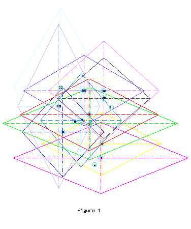
Table 3: Results
You may see the graphical representation of the result as the figure (1).
4. Conclusion
Essence of GIS motivates using fuzzy concepts. Therefore, interval approach came into attention in our concept. It seems that interval mathematics is a powerful tool for best relative placement. Interval mathematicscan be used even in general approach (quadratic programming).
The two previous approaches can be extended to optimization under inequality constraints by quadratic programming (QP). The Kuhn-Tuker theorem serves as the basis of nonlinear QP (PSHENICHNY and DANILIN,1982).
One of interesting advantage of using interval mathematics in this case study, is the manoevre field of designers. In addition, an interval will be become more general by using fuzzy boundaries. In this situation we have
[[x]]:= {[[xl] , [xu]] ½ [xl] & [xu] e RI} ; [[x]] e RII
BRPs models as well as many other models which are used in GIS, are nonlinear. The conjugate method is a suitable method, specially when inversion of matrices must be done.
Within this framework interval mathematics and best relative placement have found access to GIS. While using parallel processors and looking for best relative placement functionality, then CG method with interval mathematics work very well. Lastly, interval mathematics, the theory of conjugate method and BRP intiates a new ability for geo-spatial analysis.
REFERNCES
1. Kutterer H. (1994): Intervallmathematische Behandlung endlicher unsch?rfen linearer Ausgleichungsmodelle, Deutsche Geod?tische Komminssion Reihe C, Nr. 423.
2. Lohse P. (1994): Ausgleichungsrechnung in nichtlinearen Modellen, Deutsche Geod?tische Kommission, Reihe C, Nr 429.
3. Malek M.R. (1998): Nonlinear Least-squares Adjustement, K.N. Tossi Univ. of Tech.
4. Nickel K.(1980): interval mathematics 1980. Academic press.
5. Pshenichny B.N., Danilin Y.M. (1982): Numerical Methods in Extremal problem, Mir publishers, second printing.
6. Teunissen P. J. G. (1990): Nonlinear least-squares , Manuscripta Geodaetica, vol. 15,No.?