![]()
![]()
![]()
Modern data, for example the 1981 and 1991 censuses, publish all of their attribute data at a very spatially detailed scale, the Enumeration District, of which there are over 100,000 in England and Wales (Coombes, 1995). For earlier data, however, this is not the case. For the census of 1851 to 1961 the majority of attribute data are only available at district-level. From 1921 to 1961 this means approximately 1,800 (depending on date) Local Government Districts, while prior to this there were approximately 630 Registration Districts. Both types of district dis-aggregated into approximately 15,000 parishes and wards for which the only data published were typically the total population and the total number of males and females (see, for example, Hasluck, 1936; Lipman, 1949; Keith-Lucas & Richards, 1978). This means that most spatial detail is available for parishes while most attribute detail is available for districts. The district-level scale is, therefore, the most detailed at which it is possible to compare data over the long-term, however, even at this level it is usually impossible to compare one census with another due to the many boundary changes that occurred between them.
The Great Britain Historical GIS holds the changing boundaries of Registration Districts, Local Government Districts, and parishes as they changed from the mid-nineteenth century to 1974 (Gregory & Southall, 1998). This is linked to a large statistical database that includes data from all censuses to 1971, vital registration data (births, marriages, and deaths), and many related statistics. This means that any census data can be joined to the spatial units that were used to publish them. Unfortunately, inter-censal boundary changes make it impossible to directly compare censuses at district level over the long-term. Boundary changes can mean both the major changes in type of administrative unit used such as occurred in 1911 and 1974, and the myriad of smaller changes that have occurred piecemeal but when taken together seriously influenced the administrative geography.
In this paper the approach taken is that data should be compared at the finest level of spatial detail that is possible (Goodchild & Gopal, 1989), which, when pre-World War I data are included, means the Registration District. This has been done using areal interpolation to re-district data from all dates onto a single set of Registration Districts. Areal interpolation has been defined as "the transfer of data from one set (source units) to a second set (target units) of overlapping, non-hierarchical, areal units" (Langford et al, 1991: p. 56). It is a process that inevitably introduces a certain amount of error into the resulting data but avoids the problems of massive aggregation. Although the importance of areal interpolation as a research area has long been recognised (Fotheringham & Rogerson, 1993) there has been surprisingly little progress in this area and no single technique can be identified as better than the others. In particular, remarkably little work has been done to attempt to evaluate the degree of error that interpolation introduces.
In this paper a variety of possible methodologies are described that can be used to interpolate data from the mid-nineteenth century to 1971. In order to test the reliability of the various possible techniques, 1991 Enumeration District (ED) level data were aggregated to form synthetic units that approximated to census districts from 1881, 1911, 1931 and 1971. 1911 was taken to be the target date and data from the other three sets of synthetic units were interpolated onto these using a variety of techniques. Several different variables were used so as to evaluate the effects of their differing distributions. The results of the interpolations were then compared to the target 1911 data to calculate the degree of error introduced. The errors reveal that the effectiveness of the interpolation depends on the variable being modeled and, in particular, its relationship with total population. The choice of target unit is also very important.
The impact of this work is that it will allow continuous time-series of nearly 200 years worth of data to be analysed at district level. Although this work is applied in a historical context, it has relevance to any work that is attempting to use areal interpolation techniques.
The simplest technique used for areal interpolation is known as areal weighting. Here the data held for a set of source zones S have to be allocated to a set of target zones T. This is done by assuming that each source zones data are homogeneously distributed across their areas. Based on this assumption the data for each zone of intersection can be estimated for count or frequency data using the formula:
![]() (1)
(1)
while for data in the form of ratios, such as percentages, the formula is changed slightly to be:
![]() (2)
(2)
where ![]() is the estimated value for the target zone, ys is the
value for the source zone,
is the estimated value for the target zone, ys is the
value for the source zone, ![]() is the area of the source zone,
is the area of the source zone, ![]() is the area of the target zone, and
is the area of the target zone, and ![]() is the area of the zone of intersection between the source and target zones
(Goodchild & Lam, 1980). Models similar to this can also be used to
estimate values of Y for target zones where the target zone is assumed
to have a uniform density.
is the area of the zone of intersection between the source and target zones
(Goodchild & Lam, 1980). Models similar to this can also be used to
estimate values of Y for target zones where the target zone is assumed
to have a uniform density.
Obviously, the assumption of homogeneity is extremely unrealistic for socio-economic data. Researchers have attempted to relax the assumption using two main types of methodology: dasymetric techniques, where information about the source zones provides a "limiting variable" that provides information on the distribution of the variable within the source zone, or by using control zones where ancillary information from another set of zones, either the target zones or an external set, is used for the same purpose.
Of all the approaches in the literature, dasymetric mapping is perhaps the least developed. It attempts to make use of external knowledge of the locality to provide information on the intra-source zone distribution of the population (Monmonier & Schnell, 1984). A simple example of this is that if parts of a source zone are covered in water these should be allocated a population of zero. This technique originated in thematic mapping (Wright, 1936) and attempts to incorporate it into areal interpolation have so far been limited, however, Fisher & Langford (1995) suggest that it may be an accurate technique.
Models that use control zones take the general form:
![]() =f(x1,
x2,...,xn)
(3)
=f(x1,
x2,...,xn)
(3)
where x1 to xn are ancillary (or control) variables relating to the control zones (Langford et al, 1991).
Examples of this approach include Goodchild et al (1993) and Langford et al (1991). Goodchild et als approach attempts to use a set of external control zones that can be assumed to have a homogeneous population distribution. The population density of these zones is then estimated using a variety of regression-based techniques on the source data. Once the density of the control zones has been estimated it is used to allocated data to the target zones using areal weighting based on the population density of the control zones and the areas of the zones of intersection between the control zones and the target zones. Langford et al (1991) used classified satellite imagery to create the ancillary information. Each pixel from the image was classified as either dense residential, residential, industrial, agricultural, or un-populated. Linear regression models were then developed to estimate the population of the target zones based on the land use area within polygons with the criterion that the regression line must pass through the origin so that zones with zero area have zero population.
It should be noted that neither Goodchild et als or Langford et als models were limited by the so called "pycnophylactic criterion" (Tobler, 1979). This effectively states that data from a source zone can only be allocated to zones of intersection that lie within that source zone. An approach based on using target zones as control zones that meets the pycnophylactic criterion is described by Flowerdew & Green (1994). The technique is implemented using the EM algorithm (Dempster et al, 1977), a general statistical technique devised primarily to cope with missing data. This is an iterative process based on the expectation stage (E) in which the missing data are estimated, and the model stage (M) in which a model is fitted by maximum likelihood to the entire data set including the data estimated in the E stage. Flowerdew and Green use the idea that the zones of intersection effectively have missing data. The values for these zones can be estimated using the EM algorithm by adding knowledge from ancillary data derived from the target zones to the basic knowledge of data for the source zones and the area of the zones of intersection in a variety of ways.
A variety of differing areal interpolation techniques have been developed, therefore, based on differing assumptions and requiring differing areal units and data. Considering the amount of work that has been done, however, surprisingly little attention has been paid to quantifying the error introduced into the resulting data. Much of the work on error that has been done has been by authors evaluating their own methodology using relatively simplistic case studies (for example, Goodchild et al, 1993; Flowerdew & Green, 1994).
Sadahiro (2000) performed some detailed stochastic modeling of the error introduced by areal weighting. Perhaps unsurprisingly he found that interpolating from small source zones to larger target zones introduced relatively small amounts error. He also found that the shape of the source zones could have an impact on the results with a regular square lattice giving the most accurate results. Although Sadahiros model was sophisticated, it was based on the assumption that the underlying population were randomly distributed and, significantly, he only investigated areal weighting.
Fisher & Langford (1995) used a Monte Carlo simulation to compare different regression models developed by Langford et al (1991) to areal weighting and dasymetric mapping. They used total population from the 1991 census at ward level as source data for three Districts around Leicester. They then created random target zones by aggregating EDs using Openshaws (1977) algorithm to ensure that continuous zones were created. They agree with Sadahiros conclusion that accuracy improves as the number of target zones declines. As with other researchers they found that areal weighting was the least accurate method, but interestingly found that dasymetric mapping introduced the least error. They also found that increasing the complexity of the regression model used did improve the accuracy of the results but not very significantly. This finding perhaps contrasts with Flowerdew & Greens assertion (1994: p.134) that a simple model is more likely to be successful than a more complicated one, however, this is not necessarily a contradiction. The EM algorithm with its iterative nature and the pycnophylactic property puts more of its emphasis on the source data. The regression models developed by Langford et al, on the other hand, were designed to make the best use of detailed satellite imagery and lack the pycnophylactic criterion. This puts more emphasis on the control zones and it is perhaps unsurprising that here a more sophisticated model improves the results.
Fisher & Langfords work is expanded in Cockings et al (1997) where the mean error for a fixed set of target zones is calculated based on interpolating from multiple sets of randomly created source zones. They demonstrate that when areal weighting is used the degree of error corresponds to the geometric properties of the target zones, particularly the length of the perimeter. For their dasymetric technique, attribute properties such as the population density were more important. This is unsurprising as in areal weighting the geometries of the source and target zones are exclusively used to allocate data, whereas with the dasymetric technique attribute information is increasingly important.
Work on the error introduced by areal interpolation is, therefore, under-developed. There is broad agreement that areal weighting is the least accurate method available. It also seems clear that the amount of error introduced decreases as the number of targets is reduced. The trade-off here, however, is that detail is increasingly filtered out and modifiable areal units will become an increasing issue as this is done. Apart from Fisher & Langford (1995), Cockings et al (1997), and Sadahiro (2000), all work on error has been based on interpolating from a single set of source zones to a single set of targets. Much of the research has been focused on total population and little research has looked at the more interesting and perhaps more complicated variables that any applied analysis is likely to require. In particular, it is likely that different sub-population variables will result in different errors due to their differing spatial distributions within the underlying population surface.
![]() (3)
(3)
where ![]() is the estimated value of the sub-population variable for the parish, and
ys
is
the published value for the variable for the source zone. In the second
step, the estimated value for each target zone is calculated using a modified
version of the areal weighting formula given in equation 1:
is the estimated value of the sub-population variable for the parish, and
ys
is
the published value for the variable for the source zone. In the second
step, the estimated value for each target zone is calculated using a modified
version of the areal weighting formula given in equation 1:
![]() (4)
(4)
where Apt is the area of the zone of intersection between the parish and the target zone and Ap is the area of the source parish (Gregory, 2000).
For this technique to improve significantly on areal weighting the source districts need to be well sub-divided by their component parishes. The 1911 census provides parish-level data for both Registration Districts and Local Government Districts. There were 14,810 places, excluding wards, published in the parish-level table. There were a mean of 23 parishes per Registration District and a median of 22. There is, however, a wide range with ten Registration Districts that consisted of only one parish and a maximum of 108 parishes in a single Registration District. For Local Government Districts the distribution is significantly worse: there was a mean of 13 parishes per district and a median of only 2. While the maximum remained high at 88, less than 20% of Local Government Districts consisted of ten or more parishes while nearly half consisted of only 1. Comparing population distribution reveals a similar pattern. This is rendered even worse when it is considered that most Local Government Districts that are dominated by a single parish are urban areas and thus have relatively high populations. The conclusion from this is that a simple dasymetric technique based on parishes may well be effective in certain situations, however, it may lead to large errors in urban areas and on urban fringes where the parishes do not sub-divide districts to a satisfactory degree.
As there is no further information from the source zones that could be used to attempt to improve the interpolated estimates, using the target zones as control zones can also be considered. Green (1989) outlines how the EM algorithm can be implemented using binary, categorical, and continuous ancillary data based on the assumption that the variable of interest follows a Poisson distribution. Flowerdew & Green (1994) compared these techniques and suggest that a continuous ancillary variable introduced the least error and that a binary ancillary variable gave the most error but was still significantly more accurate than areal weighting.
In the context of the historical GIS, the use of continuous or categorical ancillary variables has been rejected for two sets of reasons. The first is the desire to emphasise the source data more strongly than the target data. It follows from this that a less detailed classification such as a polychotomous variable is less likely to have changed significantly over time than a more detailed continuous one. The second set of reasons are more practical. The M-step of the algorithm involves a model being fitted by maximum likelihood using the values estimated in the E-step as independent Poisson data. With binary data, or any other number of ordinal classes, this is mathematically and computationally straight forward, however, for categorical or continuous ancillary variables estimating the values of lj by maximum likelihood requires iterative procedures to find the maximum of the log-likelihood function (Pickles, 1985). Flowerdew et al (1991) describe how this was done by effectively allowing a statistical package, GLIM, to access GIS data from ArcInfo by modifying the object code of both packages. As modifying the object code of commercial software is beyond the scope of the historical GIS it was seen as more practical to implement the EM algorithm within ArcInfo in Arc Macro Language (AML).
Adding a polychotomous implementation of the EM algorithm to the dasymetric technique outlined above is relatively straightforward. Again, the starting assumption is that the variable of interest is evenly distributed through the populations of the source districts component parishes. This is implemented using equation 3. Equation 4 is modified to include the estimated density of the control zones and becomes the E-step of the algorithm. This gives the equation:
 (5)
(5)
where ![]() is the estimated value of the variable of interest for the zone of intersection
between the source parish and the target zone. In the first iteration all
values of lj
will be the same. In the M-step new values are estimated based on summing
the estimates of y to target zone level and estimating each value
of lambda as:
is the estimated value of the variable of interest for the zone of intersection
between the source parish and the target zone. In the first iteration all
values of lj
will be the same. In the M-step new values are estimated based on summing
the estimates of y to target zone level and estimating each value
of lambda as:
![]() (6)
(6)
The algorithm is repeated until it converges. Implementing this in AML is conceptually relatively simple although the program is computationally intensive due to its iterative nature and AML being an interpreted language (ESRI, 1993).
Any attempt to model the accuracy of areal interpolation within the historical GIS, therefore, requires a real-world, sub-parish-level geography that can be aggregated in a variety of ways to produce "synthetic" versions of parishes and districts as they existed at different dates. The data from these can then be interpolated in a variety of ways and the results compared to synthetic target zone data. Six possible methods are evaluated:
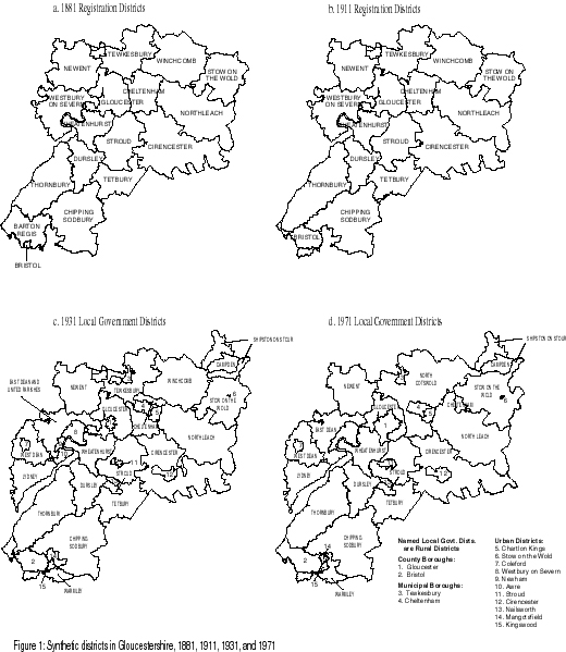
Gloucestershire was used for the test as it provides a variety of challenging situations but is sufficiently small for the results to be explored in detail. Synthetic 1911 Registration Districts were chosen to be the target districts with synthetic Registration Districts from 1881 and synthetic Local Government Districts from 1931 and 1971 providing source districts. These give a representation of interpolating from Registration Districts and from pre and post-County Review Local Government Districts. Figure 1 shows the four sets of synthetic units used. The similarity between synthetic and real units is demonstrated by comparing their areas. The mean absolute difference between real units and their synthetic versions is 8.6% with a median of 4.5%. Over two-thirds of the differences were less than 10% and the largest occurred in small urban districts. These differences will not cause artificial population densities to be created as all areas and populations are derived from complete EDs.
As well as total population, four sub-population variables were modeled: the total female population, the number of males aged between 15 and 24, the number of households with no car, and the number of households where the household head was enumerated as being in agricultural employment. This last variable was the sum of three variables from the 1991 census: "farmers - employers and managers", "farmers - own account", and "agricultural workers". The variables were chosen to provide a variety of challenges to the interpolation methodologies: the total population of the synthetic target county was 857,519 of which 50.7% were female. Males aged 15-24 made up 7.2% of the population and, from visual inspection, appears to follow the distribution of the overall population fairly well. The number of households without a car represented 11.4% of the total population but was more strongly concentrated in urban areas than the overall population distribution. Finally, the number of agricultural households, as taken from the 10% sample, represents only 0.05% of the total population and is biased towards rural areas. This means that not only does this variable show a negative correlation with the overall population distribution, it also suffers from small number problems as the target county total was only 414 agricultural households, with a minimum of 7 in Bristol target district, and a maximum of 49 in Thornbury.
Fisher & Langford (1995) used root mean square (RMS) error to quantify the error introduced in their simulations. This is based on the average differences between the estimated values of the variable and its known actual values. It is calculated using the formula:
 (7)
(7)
where ERMS is the RMS error and m is the number of target zones. They scaled this by average population to give a coefficient of variation. The population of the target zones used in the analysis presented here, however, varies widely from 250,000 in Bristol to 7,000 for Northleach and Tetbury. This means that an almost insignificant error for Bristol would have serious consequences for other districts. For this reason the RMS error formula used here calculates the proportional errors using the formula:
 (8)
(8)
In addition to an overall measure of the error, its was also felt useful
to give the maximum introduced as a proportion of the actual population.
Table 1 provides the results. 1a gives the combined results for all three
years while 1b, c, and d give the individual results for 1881, 1931, and
1971 respectively. Some experimentation was done to explore how many control
zones should be created and how they should be defined. It was decided
that four zones based on nested-means (Evans, 1977) of the target data
should be used in all cases. In some cases using eight control zones improved
the results slightly, especially where the control zones were created from
parishes. In others, where district-level data were used, two zones could
be more effective, however, the differences were not strongly significant
and it was felt that it was best to use a standard procedure as this more
accurately reflects the system as an ordinary user would use it.
|
|
|
|
|
|
|||||||||||
| RMS | Max | RMS | Max | RMS | Max | RMS | Max | RMS | Max | ||||||
| A Weight |
26.3
|
143.3
|
27.2
|
149.1
|
26.3
|
130.6
|
52.3
|
359.4
|
4.4
|
28.5
|
|||||
| Dasymetric |
13.5
|
83.2
|
13.8
|
88.0
|
13.7
|
74.9
|
35.2
|
280.2
|
14.0
|
63.6
|
|||||
| EM-District |
7.5
|
28.8
|
6.4
|
28.7
|
6.8
|
37.8
|
11.0
|
55.7
|
5.4
|
28.5
|
|||||
| EM-Parish |
5.6
|
28.6
|
5.8
|
31.0
|
5.1
|
19.8
|
11.4
|
79.5
|
14.4
|
80.2
|
|||||
| Comb-Dist |
3.6
|
22.9
|
4.1
|
23.5
|
2.8
|
14.0
|
9.9
|
48.5
|
13.9
|
62.8
|
|||||
| Comb-Par |
3.4
|
17.8
|
3.4
|
16.3
|
3.9
|
23.8
|
6.5
|
38.3
|
16.9
|
73.7
|
|||||
|
|
|
|
|
|
|||||||||||
| RMS | Max | RMS | Max | RMS | Max | RMS | Max | RMS | Max | ||||||
| A Weight |
26.1
|
84.2
|
26.3
|
82.3
|
27.2
|
88.7
|
42.2
|
120.0
|
3.5
|
9.5
|
|||||
| Dasymetric |
1.9
|
6.1
|
1.9
|
6.1
|
2.8
|
7.4
|
10.2
|
38.3
|
13.8
|
54.6
|
|||||
| EM-District |
10.7
|
28.8
|
10.7
|
28.7
|
9.6
|
26.7
|
10.9
|
38.0
|
5.9
|
22.5
|
|||||
| EM-Parish |
5.8
|
17.8
|
5.9
|
18.5
|
6.0
|
19.6
|
10.4
|
29.2
|
20.3
|
80.2
|
|||||
| Comb-Dist |
2.7
|
8.8
|
2.8
|
8.9
|
1.9
|
6.9
|
10.0
|
38.3
|
13.9
|
55.0
|
|||||
| Comb-Par |
1.9
|
7.5
|
1.9
|
7.5
|
1.7
|
5.6
|
9.8
|
38.3
|
18.5
|
73.7
|
|||||
|
|
|
|
|
|
|||||||||||
| RMS | Max | RMS | Max | RMS | Max | RMS | Max | RMS | Max | ||||||
| A Weight |
12.8
|
49.0
|
12.9
|
49.3
|
13.5
|
51.6
|
21.1
|
83.0
|
0.9
|
3.1
|
|||||
| Dasymetric |
13.1
|
50.4
|
13.2
|
50.7
|
13.7
|
53.0
|
21.6
|
85.3
|
1.0
|
3.2
|
|||||
| EM-District |
0.2
|
0.7
|
0.2
|
0.8
|
0.3
|
1.0
|
1.8
|
6.9
|
0.9
|
3.1
|
|||||
| EM-Parish |
1.4
|
5.4
|
1.4
|
5.3
|
1.6
|
6.3
|
2.4
|
9.4
|
2.9
|
11.1
|
|||||
| Comb-Dist |
1.4
|
5.4
|
1.4
|
5.5
|
1.5
|
5.9
|
1.9
|
6.9
|
0.9
|
3.2
|
|||||
| Comb-Par |
2.8
|
9.3
|
2.8
|
9.2
|
2.9
|
9.2
|
1.6
|
5.7
|
3.2
|
12.1
|
|||||
|
|
|
|
|
|
|||||||||||
| RMS | Max | RMS | Max | RMS | Max | RMS | Max | RMS | Max | ||||||
| A Weight |
40.1
|
143.3
|
42.4
|
149.1
|
38.3
|
130.6
|
93.6
|
359.4
|
8.9
|
28.5
|
|||||
| Dasymetric |
25.4
|
83.2
|
26.3
|
88.0
|
24.6
|
74.9
|
73.9
|
280.2
|
27.1
|
63.6
|
|||||
| EM-District |
11.6
|
27.8
|
8.3
|
23.5
|
10.6
|
37.8
|
20.4
|
55.7
|
9.5
|
28.5
|
|||||
| EM-Parish |
9.7
|
28.6
|
10.2
|
31.0
|
7.6
|
19.8
|
21.5
|
79.5
|
20.0
|
46.7
|
|||||
| Comb-Dist |
6.5
|
22.9
|
8.0
|
23.5
|
4.5
|
14.0
|
21.2
|
48.5
|
27.4
|
62.8
|
|||||
| Comb-Par |
5.3
|
17.8
|
5.1
|
16.3
|
6.7
|
23.8
|
8.0
|
19.4
|
28.8
|
65.8
|
|||||
d. Synthetic 1971 Local Government Districts as source zones
Table 1: RMS and maximum errors (expressed as percentages) introduced by the six interpolation techniques. Numbers in bold are the lowest errors for that variable. Key: "EM-District" the EM algorithm using the same variable for both the source and ancillary data; "EM-parish" the EM algorithm using target parish populations as the ancillary; "Comb-Dist" the dasymetric technique incorporating the EM algorithm using the same variable for both the source and ancillary data; "Comb-Par" the dasymetric technique incorporating the EM algorithm using target parish populations as the ancillary. "Farmers" refer to households whose head works in agriculture.
The results show that the combined technique usually works the best with RMS errors of typically less than 3.5% and maximum errors of less than 20%. This is the result of both aspects of the technique offering advantages in different situations: in the case of the 1881 results the dasymetric technique is far more effective then the EM algorithm, producing RMS errors of less than 3% for the three population structure variables. For the same variables the EM algorithm produces errors of around 10%. In 1931, however, this situation is completely reversed with the EM algorithm producing RMS errors of only a fraction of a percent while the dasymetric approach produces RMS errors of over 10%. These errors mainly occur in the area around Bristol: in 1881 data are being allocated from Thornbury and Chipping Sodbury source districts (and others outside Gloucestershire) to Bristol target district. The source districts are well sub-divided by parishes so the dasymetric technique performs well, only introducing small amounts of error to total population as a result of the assumption of homogeneous parish-level population distribution where parishes are sub-divided. Slightly more error is introduced into other variables because of the assumption of equal distribution of the variable through the total population. The EM approach over-estimates the population density of the zones of intersection to be allocated to Bristol target zone, either because these are zones on the urban fringe and the algorithm fails to calculate the differences in the values of l correctly, or because the control zones do not adequately reflect the complexity of the underlying population surface in these areas. The use of parish-level ancillary data improves the EM algorithm as it gives a better indication of the variations in population densities on the urban fringe, however, the relative values of l for the zones of intersection allocated to Bristol is still over-estimated. In 1931 data are allocated from Bristol source zone, which only consisted of one synthetic parish, to Thornbury target zone. The dasymetric technique, lacking any parish-level detail, fails spectacularly and over-estimates the population of Thornbury by 50% as a result of a small zone of intersection. The EM algorithm, however, copes so well with the situation that the error introduced to both target zones is less than 0.5%.
The results also show the dangers of making assumptions about the effectiveness of a technique based on the results for only one variable. They seem to show that the best results are found for total population, and that the stronger the correlation between a sub-population variable and total population the better the results of the interpolation. This is shown most strongly in the dasymetric and combined techniques where the assumption of equal distribution of the variable at parish-level is used. Where this assumption is unrealistic, particularly with lack of a car and agricultural workers, more error inevitably occurs. This causes the results for these two variables to be consistently worse than the results for the more strongly correlated population structure variables.
It is, however, hard to draw precise conclusions from these results about when it is best to use which technique. As might be expected, using parish-level ancillary data works best with total population, then with the total female population, then with the males aged 15 to 24, then those lacking a car, and finally agricultural workers. These give RMS errors of 3.4, 3.4, 3.9, 6.5, and 16.9% respectively. It might also be expected that the same trend be found using the variable itself as a district-level ancillary variable but that the errors would start higher but rise more slowly until, with some of the less well correlated variables, district-level based control zones start to give better results than parish-level ones. With the two extreme variables, total population and agricultural workers, this is the case with average RMS errors of 3.6% for total population, slightly higher than using the parish-level ancillary, and 13.9% for agricultural workers, slightly lower than using the parish-level ancillary. The results for the variables in between, however, do not follow the trend. Males aged 15 to 24 give better results using the district-level ancillary while households lacking a car give better results using parish-level data. This is unexpected but appears robust as it happens with both 1931 and 1971 source zones while the 1881 results are approximately even. It appears, therefore, that where a variable is strongly positively correlated to total population the results back up the assertion that the combined technique using parish-level ancillary data gives the most accurate results. However, with variables that do not correlate to total population as well no clear evidence is found to say whether district-level or parish-level ancillary data provide the best results.
While the combined technique gives results that appear acceptable in most cases, its results for agricultural workers are poor. This is unsurprising as the assumption of the variable being equally distributed through the total population is unrealistic. What is surprising is that areal weighting consistently performs better than the EM algorithm even when the distribution of agricultural households at district-level is used to define the control zones. This is explained by the fact that the distribution of agricultural households must be close to homogeneous within the source zones and that attempts to provide extra information on the intra-source district variation only add error.
Careful selection of target zones is an important way of reducing error. No single set of zones will be ideal for every situation so choice will depend on exact circumstances. The size of target zones is of particular importance: large targets will lead to increased loss of detail and potential problems with modifiable areal units, while smaller zones will lead to increased error from the interpolation. Another source of error that has been highlighted in this chapter occurs where data from a densely populated source zone are allocated to a sparsely populated target zone as this can easily lead to very large over-estimates of the rural target zone even when both dasymetric and ancillary information is used. This should be considered when target zones are chosen.
The most fundamental choice when selecting target zones is whether real-world units should be used or whether artificial units could be created. With real-world units, post-1974 Districts would introduce relatively little error as they are at the end of the period, thus minimising the urban expansion problems, and are relatively large as there were only approximately 330 of them. The draw-back of these is that they reduce the degree of spatial detail significantly. Selecting target zones with more spatial detail is more difficult: interpolating even Local Government District data onto Local Government Districts seems problematic due to the lack of parish-level detail underlying the more populous districts and the major differences in population densities between the urban and rural types of districts. Interpolating Registration District-level data onto Local Government Districts is not worth considering. This means that Registration Districts are the only major type of districts held in the historical GIS that would make suitable target districts. The most recent Registration Districts, those from 1911, are probably the best as these include the maximum available extent of urban areas, however, significant error is sometimes likely to be introduced as a result.
Parliamentary Constituencies provide another possible source of target zones. There are approximately the same number of these as there are of Registration Districts, however, their spatial arrangement is significantly different: constituencies are designed to have approximately equal populations and therefore sub-divide urban areas in much more detail than Registration or Local Government Districts, or even parishes, while having larger sizes in rural areas. This means that the results of interpolation in rural areas are likely to be reasonably accurate but results in urban constituencies may be error-prone. There will, however, be ancillary information available as modern census data can be aggregated to constituency level.
Where possible, creating user-defined target zones is likely to lead to lower error. A relatively simple method of doing this would be to aggregate 1973 Local Government Districts to approximately Registration District-level. From the point of view of minimising error, these would almost certainly provide more satisfactory target districts than 1911 Registration Districts as they would minimise the urban expansion problem. More sophisticated methods could also be devised that make use of the fact that all boundaries included in the system have start and end dates. This could involve starting with all boundaries that never change and then adding boundaries to these to create a set of units that seek to minimize the amount of interpolation that will result, especially where the interpolation is between two districts with considerably different population densities. This would, however, involve considerable amounts of programming and experimentation but could perhaps incorporate some of the ideas of Openshaw & Roas (1995) idea of user-modifiable units.
The combined approach advocated here attempts to make maximum use of the available data while also being sympathetic to their limitations: the parish-level population data provide much more detail on the intra-source zone distribution of population especially for Registration Districts. The use of control zones defined by data from the target date and units provides additional information especially on urban fringes where the source date parishes do not subdivide districts well. The implementation of the EM algorithm used here means that while the control zones are defined using target date data their significance in allocating data to zones of intersection is based on the source data and the use of the pycnophylactic criteria means that data from a source zones can not be allocated to zones of intersection outside that source zone.
Error in the interpolated data is, however, a fact of life. In order to minimise this the underlying assumptions of the technique must be looked at in the context of each variable used. Of particular importance is how well the distribution of the variable of interest at district-level can be assumed to follow the parish-level total population distribution. The weaker this relationship the more error that will be introduced as a result of the dasymetric technique. In cases where there is likely to be a very poor relationship then dasymetric-based approaches should not be used. A second important area is the impact of the control zones and the possibility that they may introduce bias to results for certain target zones for many dates. An example of this would be where pre-World War Two data are interpolated using modern ancillary data, new towns will have an impact on the results of certain target zones even though they did not exist at the source date. Careful choice of target zones is another way of reducing the impact of error, in particular, allocating data from source zones with large, dense populations to target zones with small, sparse populations should be avoided where-ever possible.
Even taking all this into account, however, error will still be present. This could be handled by some post-interpolation actions such as smoothing the data temporally. In addition, when interpreting any patterns produced by either analyses or visualisations of the interpolated data, the possible impact of error must be taken into account. In the longer term it is desirable that new techniques to incorporate this attribute uncertainty into both analytical techniques and visualisation of results be devised. In the case of analysis this may be through the use of Monte-Carlo simulations (Hope, 1968) or fuzzy reasoning (Kollias & Voliotis, 1991; Wang & Hall, 1996). For visualisation, some progress has been made in this area (see, for example MacEachren, 1992; Buttenfield, 1993) but, as yet this has not gained widespread acceptance.
The presence of error introduced by areal interpolation is a weakness, however, traditional analyses also contained error and inaccuracy that was usually not acknowledged. This came mainly from over-simplification. Any analysis performed at county-level lost an enormous amount of spatial detail, and thus would filter out the effects of many processes that operate at lower scales (see, for example, Savilles (1957) attempt to examine rural depopulation using a county-level analysis). Analyses that used only two snap-shots to explore change are again over-simplified when nearly two centuries of data are available. The areal interpolation approach allows national-level analyses to be performed using as much of the temporal and spatial detail as possible within the constraints of the original data source. The fact that this introduces a certain degree of error only becomes a major problem if the possible impact of this error is ignored.
B.P. Buttenfield. 1993. Representing data quality, Cartographica, 30, 1-7.
Clarke, J.I. and Rhind, D.W. 1975. The Relationship between the Size of Areal Units and the Characteristics of Population Structure. Census Research Unit Working Paper 5. Department of Geography, University of Durham.
S. Cockings, P.F. Fisher and M. Langford. 1997. Parameterization and visualisation of the errors in areal interpolation, Geographical Analysis, 29, 314-328.
M. Coombes. 1995. Dealing with census geography: principles, practices and possibilities, in S. Openshaw (ed.) Census Users Handbook, Cambridge: GeoInformation International, 111-132.
A.P. Dempster, N.M. Laird and D.B Rubin. 1977. Maximum likelihood from incomplete data via the EM algorithm, Journal of the Royal Statistical Society B, 39, 1-38.
Environmental Systems Research Institute. 1993. ARC Macro Language: Developing ARC/INFO menus and macros with AML. Redlands (CA): Environmental Systems Research Institute Inc.
I.S. Evans. 1977. The selection of class intervals, Transactions of the Institute of British Geographers, 2, 98-124.
P.F. Fisher and M. Langford. 1995. Modeling the errors in areal interpolation between zonal systems by Monte Carlo simulation Environment and Planning A, 27, 211-224.
R. Flowerdew, M. Green and E. Kehris. 1991. Using areal interpolation methods in Geographic Information Systems, Papers in Regional Science, 70, 303-315.
R. Flowerdew and M. Green. 1994. Areal interpolation and types of data, in A.S. Fotheringham and P.A. Rogerson (eds.) Spatial Analysis and GIS, London: Taylor and Francis, 121-145.
A.S. Fotheringham and P.A. Rogerson. 1993. GIS and spatial analytical problems, International Journal of Geographical Information Systems, 7, 3-19.
Goodchild, M.F. and Gopal, S. 1989. (eds.) The Accuracy of Spatial Databases. London: Taylor & Francis.
M.F. Goodchild and N.S.-N. Lam. 1980. Areal interpolation: a variant of the traditional spatial problem, Geo-Processing, 1, 297-312.
M.F. Goodchild, L. Anselin and U. Deichmann. 1993. A framework for the areal interpolation of socio-economic data, Environment & Planning A, 25, 383-397.
Green, M. 1989. Statistical Methods for Areal Interpolation: The EM Algorithm for Count Data. North West Regional Research Laboratory, Research Report 3: Lancaster.
M. Green and R. Flowerdew. 1996. New evidence on the modifiable areal unit problem, in P. Longley and M. Batty (eds.) Spatial Analysis: Modeling in a GIS Environment, Cambridge: GeoInformation International, 41-54.
I.N. Gregory. 2000, in press. Longitudinal analysis of age and gender specific migration patterns in England and Wales: a GIS-based approach, Social Science History.
I.N. Gregory and H.R. Southall. 1998. Putting the past in its place: the Great Britain Historical GIS, in S. Carver (ed.) Innovations in GIS 5, London: Taylor & Francis, 210-221.
Hasluck, E.L. 1936. Local Government in England. Cambridge: CUP.
A. Hope. 1968. A simplified Monte Carlo significance test procedure, Journal of the Royal Statistical Society B, 30, 582-598.
Keith-Lucas, B. and Richards, P.G. 1978. A History of Local Government in the 20th Century. London: George Allen & Unwin.
V.J. Kollias and A. Voliotis. 1991. Fuzzy reasoning in the development of Geographical Information Systems, International Journal of Geographical Information Systems, 5, 209-223.
M. Langford, D. Maguire and D.J. Unwin. 1991. The areal interpolation problem: estimating population using remote sensing in a GIS framework, in I. Masser and M. Blakemore (eds.) Handling Geographical Information: Methodology and Potential Applications, New York: Longman, 55-77.
Lipman, V.D. 1949. Local Government Areas 1834-1945. Oxford: Basil Blackwell.
A.M. MacEachren. 1992. Visualizing uncertain information, Cartographic Perspectives, 13, 10-19.
D. Martin. 1989. Mapping population data from zone centroid locations. Transactions of the Institute of British Geographers, 14, 90-97.
D. Martin. 1996. Depicting changing distributions through surface estimations, in P. Longley and M. Batty (eds.) Spatial Analysis: Modeling in a GIS Environment, Cambridge: GeoInformation International, 105-122.
M.S. Monmonier and G.A. Schnell. 1984. Land use and land cover data and the mapping of population density, International Yearbook of Cartography, 24, 115-121.
Nissel, M. 1987. People Count: A History of the General Register Office. London: HMSO.
P. Norris and H.M. Mounsey. 1983. Analysing change through time, in D. Rhind (ed.) A Census Users Handbook, London: Methuen, 265-286
A. Okabe and Y. Sadahiro. 1997. Variation in count data transferred from a set of irregular zones to a set of regular zones through the point-in-polygon method, International Journal of Geographical Information Science, 11, 93-106.
S. Openshaw. 1977. Algorithm 3: a procedure to create pseudo-random aggregations of N zones into M zones, where M is less than N, Environment and Planning A, 9, 169-184.
Openshaw, S. 1984. The Modifiable Areal Unit Problem. Concepts and Techniques in Modern Geography 38. Norwich: Geobooks.
S. Openshaw and L. Rao. 1995. Algorithms for re-aggregating 1991 Census geography, Environment and Planning A, 27, 425-446.
S. Openshaw and P.J. Taylor. 1979. A million or so correlation coefficients: three experiments on the modifiable areal unit problem, in N. Wrigley (ed.) Statistical Applications on the Spatial Sciences, London: Pion, 127-144.
Pickles, A.R. 1985. An Introduction to Likelihood Analysis. Concepts and Techniques in Modern Geography 42. Norwich: Geobooks.
Y. Sadahiro. 2000. Accuracy of count data transferred through the areal weighting interpolation method, International Journal of Geographical Information Science, 14, 25-50.
Saville, J. 1957. Rural Depopulation in England and Wales: 1851 to 1951. London: Routledge & Kegan Paul.
W. Tobler. 1979. Smooth pycnophylactic interpolation for geographical regions, Journal of the American Statistical Association, 74, 519-530.
F. Wang and G.B. Hall. 1996. Fuzzy representation of geographical boundaries in GIS, International Journal of Geographical Information Systems, 10, 573-590.
J.K. Wright. 1936. A method of mapping densities of population with Cape Cod as an example, Geographical Review, 26, 103-110.