Improving Snakes for Linear Feature Displacement in Cartographic Generalization

Mats Bader and Mathieu Barrault
Spatial Data Handling, Department of Geography
University of Zurich
Winterthurerstrasse 190
CH-8057 Zurich, Switzerland

E-mail: mbader@geo.unizh.ch , barrault@geo.unizh.ch

Abstract

Cartographic generalization is a demanding element of map making. Attempts to display data at scales smaller than the source can result in spatial conflict, whereby map symbols become too close or overlap. Several map generalization operators may be applied to solve the problem. One of these operators is displacement, where objects are moved and/or deformed in the attempt to resolve proximity conflicts between objects. Displacement of lines is especially demanding, as a line can not be shifted as one rigid object. A displacement applied to a part of a line needs to be spread out and cushioned within the line. This subtask in road displacement is called propagation. To model propagation, we treat lines as snakes - a widespread technique in computer vision - and enhance this model to honor cartographic constraints. Therefore we change the underlying energy definition of snakes, making the stiffness of lines mirror the road shape and expand the approach such that the algorithm works on entire road networks. The resulting algorithm performs good and robust propagation and is the basis for a global displacement algorithm based on the same fundamental considerations of energy minimization.

1. Introduction

Problems arise when the user requires a map at a scale significantly smaller than that associated with the source data. Typical consequences of displaying pre-generalized data at a smaller scale than originally intended are that the detail of individual map features may become too small to be legible, while neighboring symbols that should be clearly distinguished may become too close or they may overlap each other. These latter problems of graphic conflict arise in particular when the map symbols are no longer true to scale of the features they represent.

Both in traditional and computer-aided generalization, many operators have been identified. Line simplification is probably the best studied operator. In recent years special attention was paid to displacement. Displacement is necessary mainly due to increased symbol width of roads. The road symbols may be much wider, when map scale is taken into account, than the width of the road on the ground.

In this field of research mainly two types of displacement problems are discussed. First the relocation of buildings in a road partition is studied. Due to the increased width of the road symbol and the increased minimal distance between objects, buildings need to be shifted away from the road. This task becomes considerably complex if the free space is limited by other roads. A second type of algorithms intends to solve conflicts between roads. Such conflicts are resolved by shifting and deforming conflicting line fragments. In this article we focus mainly on propagation - an important step in the displacement process of such line conflicts.

1.1 Definitions and Constraints

A line consists of a set of ordered vertices connected by straight line segments. The first and last vertices in a line denote nodes. Intersection nodes are those nodes which are shared by more than two distinct lines. End-nodes belong to one line only.

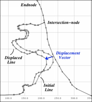
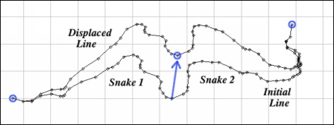
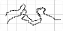
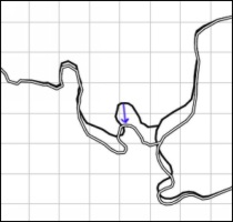
The trigger for propagation is a displacement vector applied to a vertex within a line (see Figure 1). In the generalization process such a displacement vector is often the result of a previous algorithm specifying the amount and direction of displacement that would resolve a proximity conflict between two lines in the conflict spot. [However, the displacement vectors in the illustrations of this paper are specified by the user and are not the result of any computation.]

Figure 1: Initial line and displaced line after propagating a displacement through the line. Propagation is the act of diffusing and cushioning a displacement offset in the line, see Figure 2. Propagation is influenced by two factors.
1. The character of a line would be heavily distorted if applying the displacement to a single vertex only. In order to preserve the shape of a line, the neighborhood of the displaced vertex needs to be displaced too. The shape would be preserved perfectly if all of the line's vertices could be moved by the same offset.
2. Any shift of vertices decreases geometric accuracy and raises the danger for new conflicts due to object interference.

Displacement propagation needs to balance those conflicting constraints. The aim is to limit the propagation such that the character of the targeted line is preserved within a minimal cushioning distance. It is the cartographer who judges whether small shape distortion at the cost of reduced geometric accuracy is more important than higher precision at the cost of higher shape distortion.

Correction of geometry without propagation

Figure 2: Roads in conflict due to symbol overlap (left). Applying only a correction to the interfering vertices gives unacceptable results (middle). The displacement has to be propagated throughout the line (right). In addition to this fundamental dichotony, propagation needs to respect some additional basic constraints. Propagation must not introduce any self-intersections or symbol overlaps in a line. Further a smooth transition between displaced parts and the original line has to be ensured. These constraints are handled intuitively in manual generalization. But they need to be formalized and handled properly when automating generalization.

We denote these constraints as intra-line constraints. Such constraints can be evaluated taking only one line into consideration. Many more constraints come into play when we include inter-line problems. Such constraints describe the behavior between lines. We distinguish two types of inter-line problems. On the one hand, lines must be treated together if they are connected. If a line in a connected network is moved, the network has to react to this shift to avoid loss of connectivity. We will discuss such problems in Section 3. On the other hand, lines interact if they share any special spatial relationship, such as proximity and alignments. In this paper we do not respect such problems.

1.2 State of the art

Propagation is mainly treated as a subtask in cartographic displacement. For over a decade the algorithm by Nickerson (1988) was the best studied displacement algorithm. A line is chosen for displacement based on a ranking of conflict types. For every vertex of that chosen line a displacement vector is computed. To retain the shape of the original line, two modifications are made to the displacement vectors. First, they are modified such that they all correspond to the same direction. Secondly the displacement magnitudes are filtered to avoid rapid changes. Having implemented Nickerson's algorithm in a platform such as AGENT (Lamy et al., 1999), we found that this algorithm does not satisfy our requirements. It is difficult to find good parameters to use the algorithm. For each conflict the parameters have to be readjusted. The preliminary results are poor from a cartographic point of view and so the algorithm is deemed to have serious deficiencies.

Recently researchers started tackling the problem in a different way. Instead of deriving displacement sequence, displacement direction, displacement magnitude and propagation in a sequence of tedious steps, displacement is regarded in a more global sense and is modeled as an optimization problem. E.g. Harrie (1999) minimizes the violation of geometric constraints which describe the shortcomings of a map, using a least squares method. Other researchers brought up energy minimizing techniques based on variational principles. Højholt's (2000) approach stems from solid mechanics. He models the map space as elastic material. The method is very promising for area displacement, but lacks from possibilities to integrate the character of lines. Burghardt (1997) adopted the technique of snakes for displacement. We will describe the basics of snakes in the next section and improve the model for cartographic displacement.

1.3 Goals

As propagation is only a part of displacement, the reader might ask why we treat this step in isolation.
First, only a thorough understanding and good model of the propagation process enables us to build a powerful displacement algorithm. So we understand this article as contribution to the improvement of displacement algorithms, especially ones based on snake techniques.
Second, propagation is not only useful in the displacement process, but is also an often necessary operation in combinations with other operations to cope with side-effects. Not only displacement does change the position of line fractions, e.g local enlargement of bends also poses the difficulty of reconnecting inner partitions of lines which make a subsequent propagation necessary. A satisfying method for this does not yet exists. Particulary, we need a robust method, producing cartographic good results, which does not require a complex parameter configuration.

Thus the goals of this article are twofold: Enhance the adaption of the snake technique for cartographic generalization - a key requisite to a global displacement method; And present a robust, easy to handle and universally applicable algorithm for propagation. While displacement deals with the conflicts arising between lines, propagation is limited to intra-line shape preservation.

In the next section we present the idea of snakes. The basic model is enriched in Section 3 to honor additional cartographic requirements, followed by a general outlook.

2. Snakes

Snakes are a special case of deformable models. They were proposed by Kass et al. (1987) in the field of computer vision. The aim of the method in its initial form was to extract smooth shapes in a given region of a a raster image. The idea is to introduce an elastic curve (line) in the image, and let it evolve from an initial position under the action of internal forces (smoothness constraints) and external forces (attraction towards salient edges). Under these forces the line meanders towards a position of minimal energy. This movement resembles the one of a snake - that's where the method derived its name.

We formulate directly the model adopted to cartographic line treatment and recall some definitions. Let denote a line of length . We define displacement as a mapping

$\begin{displaymath}s \mapsto d(s) = \left( x(s)-x^0(s), y(s)-y^0(s) \right)^T\mbox{ , } 0 \leq s \leq l\end{displaymath}$

where denote the coordinates of the initial line and , give the coordinates of the displaced line. So is a parameter representation of the displacement between the initial (original) line and a derived (displaced) line. We define a deformable model as a space $\cal{A}$ of admissible deformations of the line and a functional representing the energy of a deformation.

$\begin{displaymath}E: \cal{A} \mapsto \mathbf{R}\end{displaymath}$

(1)

This functional represents the energy of the model and has the form

$\displaystyle E(d)$	$\textstyle :=$	$\displaystyle \int_l{E_{tot} ds}$
	$\textstyle :=$	$\displaystyle \int_l{ \left(E_{int}+E_{ext} \right) ds}$
	$\textstyle :=$	$\displaystyle \int_l{ \frac{1}{2} \left(\alpha(s) \vert d'(s)\vert^2 + \beta(s) \vert d''(s)\vert^2 +E_{ext} \right) ds}$	(2)

where and denote derivatives of with respect to and where $E_{ext}$ is a potential associated with external influences (see below). The aim of the method is to find among all admissible deformations $\cal{A}$ the deformation that minimizes this energy.

Inner Energy In contrast to classical snakes in computer vision, the inner energy defined in (2) does not mirror the geometry of a line, but measures the difference between two lines - the initial line and its geometry after propagation. Deviations of first and second order derivatives are used as quality measures. Such a treatment was proposed by Radeva et al. (1995) to incorporate structural information of objects in object recognitions. We owe the basic snake approach in cartographic generalization to Burghardt (1997). The properties of the model are controlled by the parameters $\alpha(s)$ and $\beta(s)$ . Their choice determines the elasticity and rigidity of the model. A discussion of these values is subject of Chapter 3.

External Energy The outer energy is an arbitrary value that penalizes (or rewards) a current deformation of the line based on external criterias. E.g we could penalize a deformation when two neighboring lines get in conflict due to an intended shift. The power of snakes lies to a big part in this interplay between external forces, pushing a snake towards admissible places of interest, and internal regularization forces, making the line resemble its initial form. For this article we do not use any external energy. We give an outlook of this promising interplay in Section 4. As pointed out in section 1.1, we focus on intra-line problems which are guided by the line's inner energy only. A thorough understanding of the inner energy is a key step towards a global displacement method.

The space of admissible deformations $\cal{A}$ in (1) is restricted by the boundary conditions , , , , which define the displacements and line direction at the snake's head and tail. The aim is to minimize the energy stored in the line defined by the distance function subject to these imposed boundary conditions. These values define the best displacement.

According to the calculus of variations, is a local minimizer for if it satisfies the associated Euler-Lagrange equations

$\begin{displaymath}\renewedcommand{arraystretch}{1.2} \left\{\begin{array}{l......\mbox{given } d(0), d'(0), d(l), d'(l)\end{array} \right.\end{displaymath}$

(3)

Here we already removed the external energy term which we assume to be zero. This is a pair of two independent differential equations of fourth order. It is solved for the

-direction, setting

, and the

-direction using

Factoring out deformation dependent external energies makes the solution easier, as we can avoid an iterative solution. Because we can solve (2) without iteration, no snake is wiggling through the map. Nevertheless we maintain the name 'snake', as the definition of the inner energy is characteristic for snakes in computer vision and because the model can easily be extended again to incorporate external effects.

For the numerical solution of the partial differential equations we used a finite element method (FEM). Our implementation follows the ideas by Cohen and Cohen (1993), whereby line segments define a natural tesselation of the line. We did choose first-order (cubic) Hermitian polynomials as basis functions. The finite element method leads to a linear eqaution system $\mathbf{A v = 0}$ , where the matrix is symmetric, positive definite and pentadiagonal. From the solution $\mathbf{v}$ , we can derive the necessary displacements.

If we apply the method with zero-boundary conditions, a valid solution for $\mathbf{v}$ is $\mathbf{0}$ . The resulting function is vanishing. So no displacement is applied if the snake is activated with vanishing displacements at the end. Of course we apply usually non-vanishing boundary conditions to one end, as we use a predefined displacement vector in the conflict spot as fixed tail of the snake, limiting the space of admissible deformations $\cal{A}$ to such deformations that perform the required displacement.

We also tested a finite difference approximation, see Kass et al. (1987), Neuenschwander (1995) and Burghardt (1997). For equidistant and dense point sampling both methods work well and produce similar results. For irregular point sampling - which we encounter often in digitized roads - and large segments, the FEM is better suited. The results do not vary with the sampling, but with the shape of the line only.

3. Improving the method

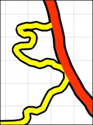
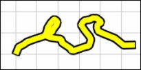
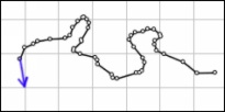
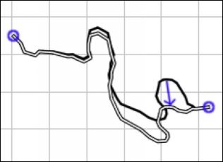
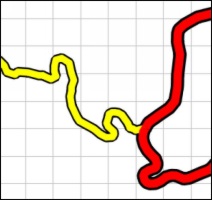
Figure 3 shows the application of snakes for displacement propagation. Throughout the paper, arrows in figures indicate a user defined displacement which is imposed as boundary conditions to one side of the snake. Such a displacement vector is usually the result of a previous algorithm based on an analysis of the conflict area. Circles mark places where the snake is fixed at places on the initial line. So in Figure 3 we applied two snakes. Both snakes have their tails fixed to zero displacement somewhere on the initial line and the head fixed to the desired displacement. We incorporate boundary conditions such that the direction of the snakes head and tail stay the same as they were on the initial line. Thus we can ensure smooth transitions (first order continuity) between the snakes. Of course, it does not matter which end is the head and which is the tail of a snake. We just use these terms to distinguish the two ends of the snake.

Figure 3: A line is split by the displacement vector into two parts. For both parts a snake algorithm is invoked. One side is fixed to the initial line and the other end is set to perform the required displacement. The presented method works well, in principle. The snake approach preserves local and global shapes well. The boundary conditions are respected. No additional adaptations are necessary to fulfill smooth connections to the surroundings. It is worth reviewing what the method does. If we take one end of a line and displace it, the method will find a function of displacements, minimizing its first and second order derivatives. This minimization is done in the

and

direction separately. The parameters $\alpha$ and $\beta$ define the importance of the first, resp. second order derivative in the minimization.

Even though the results are fine in the above example, the approach violates important cartographic requirements:

(1): The result of propagation depends on the position of the snake's tail. While the head is defined by the position of the applied displacement vector, the tail can be placed at any arbitrary position along the line. Wherever the tail is positioned, propagation will finish there. The entire length of the line is used to cushion the displacement. So the result depends on the choice of the tail's position.
(2): The characteristics and type of a line do not enter into the computation. Exaggeration is more easily applied on complex (very sinuous) lines. Applying a displacement to a straight highway is much more of a problem - propagation must be performed carefully, using a greater length to cushion the displacement.
(3): The snake technique allows self-intersection, not guaranteeing an absence of symbol overlap.
(4): If a displacement vector is applied to a line close to an intersection, cushioning is not possible in the affected line only. A propagation algorithm must have the ability to spread a displacement over junctions as well.

We present solutions to overcome these drawbacks. (1) is guaranteed by changing the underlaying energy definition. A shape related setting of the parameters $\alpha$ and $\beta$ will solve problem (2) and (3). Finally we constitute a system to include more than one snake only, which results in a solution for (4).

3.1 Attraction term

As pointed out above, cushioning displacement is done using the entire length of a snake. Therefore the result depends on the choice of the snake's tail. Finding automatically a good position for this tail is demanding. We prefer a method which could take any arbitrary point far enough from the snake's tail and which would cushion the displacement within as little of its length as possible - always subject to the constraint of shape preservation. Then we would get rid of a search for admissible snake endpoints and obtain predictable results.

To achieve this goal, we extend the standard snake model by an attraction term.

$\begin{displaymath}E(d) = \int_l{ \frac{1}{2}\left(\psi \vert d(s)\vert^2 + \alpha \vert d'(s)\vert^2 +\beta \vert d''(s)\vert^2 \right) ds}\end{displaymath}$

The $\psi$ -term is added to the internal energy (2) and penalizes the line as long as it does not coincide with the original position yet. As a consequence, the line strives to fall back to its initial position. The higher the value for $\psi$ , the higher positional accuracy is assessed in comparison to the shape parameters $\alpha$ and $\beta$ .

Incorporating this additional term is straightforward. Applying the Euler-Lagrange equation we obtain

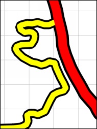
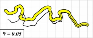
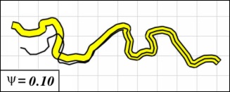
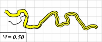
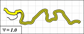
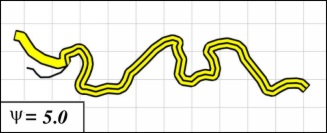
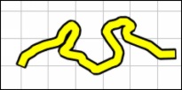
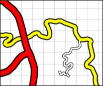
$\begin{displaymath}\psi d(s) - \alpha d'(s) + \beta d''(s) = 0\end{displaymath}$

In Figure 4 the results of applying the improved propagation is shown using different values for $\psi$ . We can now choose any point on the line as the tail of the snake and get the same result. The line will fall back to its initial position as soon as possible. Only a subset of the entire snake length is used to cushion the displacement. We can always use the line's endpoint as a snake limiting extent and do not have to consider about the claimed extent of cushioning. Of course, this is only true if the line is long enough to incorporate a specified displacement. If the line is too short, resp. a displacement offset is required close to the line's endpoint, the method mismatches the displacement. The displacement changes the character of the line. We return to this point in Section 3.3.

Figure 4: Displacement applied to the left of the line with fixed right endnode and different values for psi. As reference, the thin black line displays the original position. Increasing psi makes the displaced line return faster to its original position.

3.2 Adaptive $\alpha$ and $\beta$

As stated in Section 1.1, propagation aims at cushioning a displacement without changing the perceived characteristics of a line. The presented technique does not yet respect any peculiarities of a line or displacement. We improve our model to solve the following cartographic requirements:

(1): From a cartographic point of view, straight lines are harder to deform than sinuous ones. Deforming a very sinuous line is hardly noticed by the user, while altering the shape of quasi straight lines changes the perceived character remarkably. Introducing bends in straight lines is prohibited.
(2): The elongation (or shrinking) of a line to absorb a displacement is divided by all segments. Generally, this is a good property of snakes. However, we would improve quality if straighter parts of roads, which have approximately the same direction as the desired displacement, would absorb more of the displacement. Such a behavior improves geometric accuracy, as the displacement is cushioned sooner. This approach is motivated by the fact that a change in length of long parts is hardly noticed by the map reader, as it does not change the characteristics of the line.
(3): If we displace the end of a line with sharp bends in direction perpendicular to the bend axis, the road symbol may overlap after propagation (see Figure 5). Important bends should be protected form being squeezed.

Improvements are integrated by varying $\alpha$ and/or $\beta$ . To overcome problem (1), we characterize each road before we apply our algorithm. Based on road attributes (e.g. highways are stiffer than agricultural roads) and sinuosity measures, we assign different values to $\alpha$ and $\beta$ for the whole line. High $\alpha$ / $\beta$ -values make the snake more resistant against deformation. As long as we restrict the algorithm to individual lines, an increase of the shape parameters $\alpha$ and $\beta$ has the same effect as if we decrease the attraction term $\psi$ and hold $\alpha$ and $\beta$ constant. Sill we recommend adjusting the shape parameters rather than $\psi$ . First, from a ideological point of view, we characterize the lines, so we should change the shape parameters rather than the $\psi$ -term used to quantify positional accuracy. Second, when we extend propagation to a whole network, the propagation will be shared based on the deformation resistance. Finally the behavior of the line against deformations becomes crucial when including forces into the system.

For problem (2) we change the parameters within each segment. We decrease $\alpha$ and $\beta$ for those parts of a line which are oriented in displacement direction. Such a treatment makes these segments shrinking or growing such that they absorb more of the displacement magnitude. This approach is only useful for segments that are oriented in displacement directions, as other segments would be modified in a unacceptable way. They would compensate a desired displacement by changing their direction. This is no problem for segments placed in displacement direction, as they have no motivation to change their initial bearing.

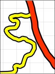
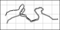
Finally we protect any important feature of the line by increasing $\alpha$ and $\beta$ drastically in these segments. This keeps the shape of the detected feature untouched. In Figure 5 results with the improved technique are illustrated.

Figure 5: The propagation in a line can lead to cartographically unacceptable deformations (middle). Critical parts can be protected by raising alpha and beta (right). From the physical interpretation of the model, one might expect that we can comnrol the behavior of the snake along the segment lengths by the first derivatives and influence the bending by the second derivatives. However, we usually increase (or decrease) both $\alpha$ and $\beta$ together. Experimental tests showed that the results are not very sensitive to any relative exaggeration of $\alpha$ and $\beta$ . Control is only gained when increasing the magnitude both for $\alpha$ and $\beta$ , but not their balance. This restricts our possibilities to guide the displacement. On the other hand we do not have to consider the initial choice of $\alpha$ and $\beta$ and can get rid of a sensitive parameter.

3.3 Handling junctions

Not every displacement can be cushioned within a line. Applying a displacement to a line close to a junction poses major problems. Cushioning with fixed endnodes might change the characteristics of a line in an inadmissible way. We prefer a method where no endnode must be fixed. Even though a line should be inclined to reach its original position, there is no compulsion to do so. If the shape does not allow cushioning the displacement before the end of the line, also the endnode can and should be displaced.

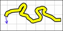
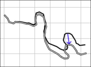
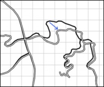
This new demand is met by identifying a line as one snake only. The desired displacement is applied to an interior vertex of the snake. For the head and tail no displacement is prescribed. As we incorporated a $\psi$ -term, the head and tail gravitate to their initial position by themselves (see Figure 6).

Incorrect propagation due to lack of space for correction

Correct propagation with displacement of endnodes

Figure 6: A displacement applied close to an endnode leads to cartographically unacceptable results if the endnodes are kept fixed (left). Endnodes can be freed due to the psi-term. This allows endnodes to move, if necessary (right). Having this approach in mind, we are able to treat propagation for the entire road network. The easiest way to do so is to apply snakes successively. Whenever an intersection-node has to be moved due to a displacement, we run the snake algorithm for all other lines connecting to this intersection.

Another, more global approach is to handle the entire network simultaneously. Consider a connected set of lines. We allow the junctions to move, but assume the set is chosen such that any displacement can be cushioned without moving the endnodes (see definitions in 1.1). We model each line as individual snake. For each snake we can build a linear equation system as sketched in section 2. We do not use the extended $\psi$ -model and do not yet impose any boundary conditions to this equation system. So the resulting snake matrix is singular and thus the linear equation system has no solution. This is no surprise, as no best configuration can be found if we do not define a displacement nor a fixing to the line-ends. In a next step we assemble all the single snake matrices in a huge matrix, which defines the entire road network. When snakes join nodes - which happens in all intersections - the values of the matrix cells are just added. So, a displacement of the intersection node affects all lines ending in the said node. Finally we impose the boundary conditions on the global matrix. Every endnode is fixed and the required displacement is included in the matrix.

This modification enables us to compute propagation for an arbitrary placed displacement vector in the road network. For the sake of simplification and computer power, a partitioning of the road network is usually applied before starting any generalization algorithm. These partition boundaries have to stay fixed to ensure smooth transitions between them. Therefore we applied no displacement to the endnodes in above description.

The scope of this paper unfortunately does not allow a detailed discussion of the advantages and drawbacks of the two proposed techniques.

Figure 7: A displacement applied close to an intersection needs to be propagated through the neighboring roads.

3.4 Results

Figures 3 - 8 show some results of our method. The modifications proposed in this section are incorporated. The algorithm produces cartographically satisfying results, that is propagating any given displacement through a network of roads. The algorithm works equally well with multiple displacement vectors, although only a single vector is illustrated in the figures.

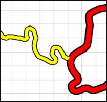
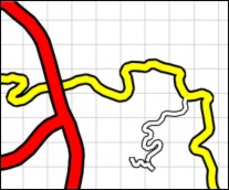
Applying the algorithm to connected roads meets the cartographic demands (see Figure 8). Junctions move with more resistance, as they pass on the shifting to two or more other lines. Due to different settings of the shape parameters $\alpha$ $\beta$ , displacement is strongly cushioned in the sinuous line to avoid passing over a displacement vector to the rigid main roads.

Figure 8: Propagation is computed for all lines in a road network simultaneously. Due to the higher stiffness of the main roads to the left, displacement is strongly cushioned in this direction. To the right of the applied displacement vector there is no need for strong cushioning. As the method is based on a solid mathematical model, it is very robust and never crashs. The method also handles major displacement values.

The process is guided using a single parameter $\psi$ . This parameter allows the map producer to weigh requirements concerning positional accuracy against shape distortion. If set once, the parameter is generally valid for an entire map series. Reference values for $\alpha$ and $\beta$ are set internally. The initial absolute values are mostly arbitrary. The relative magnitude with respect to each other determines the sensitivity of lines.

Results do not depend on the sampling scheme and density of the line. Therefore we do not have to introduce auxiliary points to support the computation. We keep the amount of vertices low. Results were generated on a testbed implemented in Java on a Sun Ultra 30. Computing resources are mainly consumed by the Cholesky factorization to solve the linear equation system. We integrated a Cholesky factorization which does not respect the sparseness of the matrix. Note that the pentagonal structure of the global matrix is destroyed when handling more than one snake. Nevertheless, computation of up to 200 vertices is performed in less than a second.

4. Conclusion and Outlook

This paper presented an algorithm for displacement propagation in cartographic line displacement. The method is based on snakes, a technique introduced to generalization by Burghardt (1997). The underlying energy definition was changed to perform fast cushioning of displacement. A special assembly of several snakes was presented which allows extending the method for entire road networks. The result of a preceding analysis of line shape and characteristics is translated into the model via setting model inherent shape parameters.

Our model does not include any external energy yet. Burghardt (1997) already presented a method to handle displacement using snakes. For each line a displacement potential is computed based on proximity measures. In the conflicting areas, forces are applied to the snakes which push them away from the conflict spots. The snakes iteratively leave the area of conflicts. The propagation of such a displacement is guided by the inner energy. Our proposed modification of the snake improves the quality of such solutions. The characterization of lines, resulting in different resistance against deformations, helps to make the best suited roads move. Our future goals include describing a global method for road displacement on an entire road network, based on these modifications.

Acknowledgment

This research was supported by the European Union Information Technologies Programme ESPRIT No. 24939 (AGENT).
Thanks go to R. Weibel for valuable assistance and F. Brazile for general comments.

References

Berger M.D. (1991): Les contours actifs: modélisation, comportement et convergence. Doctorat de l'Institut National Polytechnique de Lorraine.

Burghardt D. and S. Meier (1997): Cartographic Displacement using the Snakes Concept. In: Foerstner W. and L. Pluemer (eds): Semantic Modeling for the Acquisition of Topografic Information from Images and Maps. Birkhaeuser-Verlag, Basel, Switzerland.

Cohen L.D. and I. Cohen (1993): Finite-Element Methods for Active Contour Models and Balloons for 2-D and 3-D Images. IEEE Transactions on Pattern Analysis and Machine Intelligence, Vol. 15, No. 11, pp. 1131-1147.

Harrie L.E. (1999): The Constraint Method for Solving Spatial Conflicts in Cartographic Generalization. Cartography and Geographic Information Science, Vol. 26, No. 1, pp. 55-69.

Huebner K.H., E.A. Thornton and T.G. Byrom (1995): The Finite Element Method for Engineers. Third Edition. John Wiley & Sons.

Højholt P. (2000): Solving Space Conflicts in Map Generalisation: Using a Finite Element Method. Cartography and Geographic Information Science, Vol. 27, No. 1, pp. 65-74.

Kass M., A. Witkin and D. Terzopoulos (1987): Snakes:Active Contour Models. Proceedings of the First International Conference on Computer Vision. IEEE Computer Soc. Press, pp. 259-269.

Lamy S., A. Ruas, Y. Demazeu, M. Jackson, W. Mackaness and R. Weibel (1999): The Application of Agents in Automated Map Generalisation. Conference Proceedings ICA, Ottawa, Canada, pp. 1225-1234.

Neuenschwander W.M. (1995): Elastic Deformable Contour and Surface Models for 2-D and 3-D Image Segmentation. Dissertation, Swiss Federal Institute of Technology (ETH) Zurich, Switzerland.

Nickerson B.G. (1988): Automated Cartographic Generalization for Linear Features. Cartographica, Vol. 23, No. 3, pp. 15-66.

Radeva P., J. Serrat and E. Marti (1995): A Snake for Model-Based Segmentation. Fifth International Conference on Computer Vision, IEEE Computer Society Press, Los Alamitos, California. pp.816-821.