![]()
![]()
![]()
Vertical simple shear is usually adapted to set up the boundary conditions because it facilitates the calculations.
Nevertheless, in the program is used a Mathematica®-built displacement direction function consistent with inclined simple shear conditions.
To find the derivatives of the displacement direction function, an essential sub-routine in the simulation, two approaches are used. The first involves a numerical solution based upon the Crank-Nicholson method. The second requires the calculus of the derivatives with the support of Mathematica® built-in functions.
A brief analysis is carried out on the graphical display of these sub-routines.
An assesment on the efficiency of Mathematica® for linear finite-element modelling is given based upon the availability and efficiency of resources found in the system during the programming of the algorithms.
The graphical and analytical capabilities of Mathematica® are used to generate the trajectories and velocity fields of the hanging wall particles with respect to an Eulerian system of reference.
Key words: Hanging Wall Deformation, Simple Shear, Finite Difference,
Crank-Nicholson.
Volume balance is achieved as a consequence of constraining the deformation to incompressible conditions, but the effects of compaction (Waltham, 1990) and density increase with depth (Waltham, 1992) can be included to support more elaborated models.
This forward modelling is specially useful for the interpretation of
seismic data from fault zones, that are known to be of poor resolution
(Kerr and White, 1994).
Comparing the simulation of deformation associated with a variety
of fault shapes with either the deformation of the overburden above
the fault zone or the one of the faulted sequence makes feasible
to deduce the real fault geometry, partial o totally faded in the seismic
record.
For oil business purposes this branch of computer modelling is now of
increase demand since makes possible valid and reliable interpretations
of the boundaries of faulted reservoirs (Kerr and White, 1996). The impact
of this fact is felt specially for a reliable calculation of the volume
of such reservoirs and for the plans of well drilling toward its
boundaries.
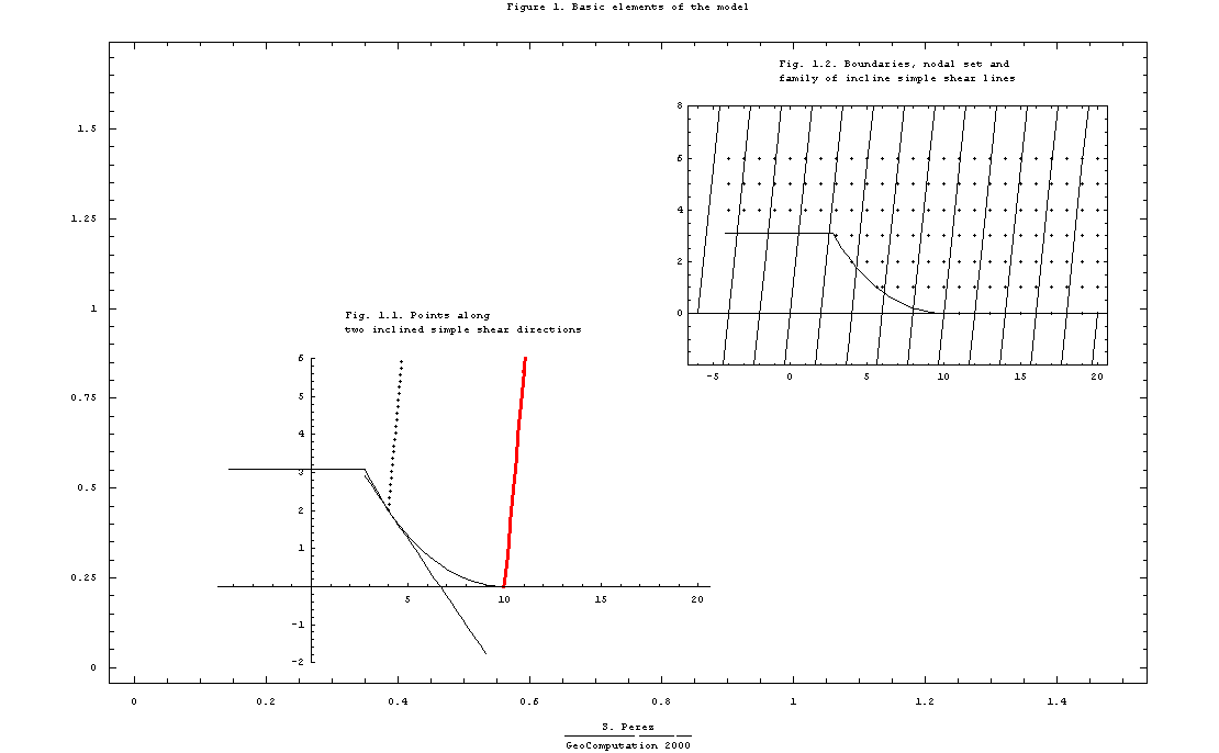
The coordinates of the nodal points in the hanging wall can be arranged in tables using the respective Mathematica® facilities.
The points along the isogons (-20 degrees of slope) would have a displacement direction parallel to the tangent to the fault at its intersection. In Figure 1.1 are represented the points along the isogon y=5.67(x-4)+2 (black dots) and the isogon at the boundary between the horizontal line (detachment) and the curved section of the fault . That isogon correspond to the line y=5.67(x-10). The line separates the displacement directions of zero angle from those continously decreasing along the circumference. The fault would sole out in a horizontal plane above which horizontal layering would be represented joining the plot of a nodal set of points prior to deformation (Fig. 1.2). The horizontal line between the ordinates 3 and 4 would be a detachment surface during inversion (see Fig. 7.2)
Mathematica® allows to obtain the displacement direction for any point in the hanging wall by the means of a piecewise function, defined analytically following the conditions of inclined simple shear .
That function is subsequently used for the calculations involved in the Crank-Nicholson method and to define, later on, the position of hanging wall nodes as its deformation evolves.
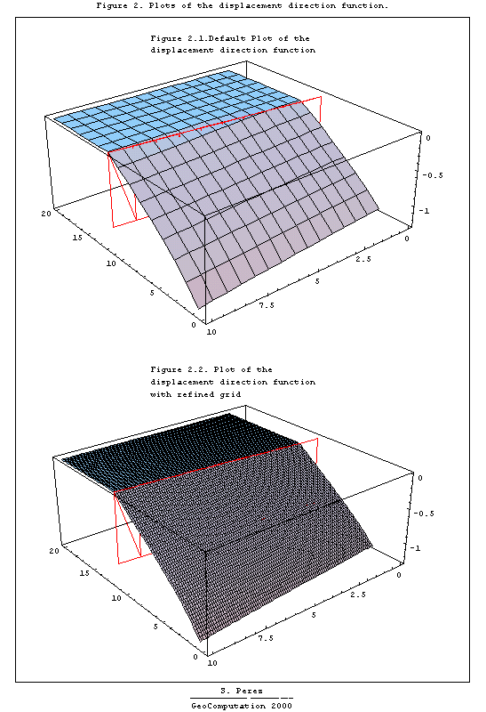
From Figure 2.1. is possible to identify a zone of subtle torsion in the surface. Is located around the boundary between the horizontal line and the circumference. In the model corresponds to the change between inclined simple shear angle domains, from 0 radians to the region where depends upon the slope of the tangent to the circumference.
The real boundary between the displacement directions domains is an
inclined simple shear line. In Figure 2 is the
line at the top of the vertical plane, outlined in red, above the
surface. That line corresponds to the equation
y =5.67(x-10), and is the inclined simple shear line at the intersection
between the detachment and the listric section of the fault.
The region of torsion in the surface is in reality an artifact due to the combination of two factors:
1) The inclination of the simple shear lines does not make the correspondence of angular values for the points in the domain parallel to the Y-axes.
2) For graphical purposes, Mathematica® uses a default grid size, and interpolates the function between the points located in the grid. As a matter of fact, the Mathematica® default sample interval cross the real boundary (y=5.67(x-10)) between the displacement direction domains, as is seen in Figure 2.1.
A better graphical approach to the function is reached if the plot is made based upon a smaller interval size for the grid than the default one. In Figure 2.2. is appreciated that the smaller interval grid size allows an approach of the plot to the real surface boundary at y=5.67(x-10) that is closer than the one given by the default grid.
The boundary conditions for the velocity field are set up following Walthams guidelines. Of particular interest is the fact that at the boundary lateral side of the model a constant horizontal velocity, either of extension or normal inversion, is endowed.
The magnitude of the unknown velocity field is calculated from
the system of linear equations generated from the partial differential
equation that governs the model. In other words that implies to find a
solution of the Laplace Equation for potential flow (Harbaugh and Bonham-Carter,
1970; Waltham, 1989):
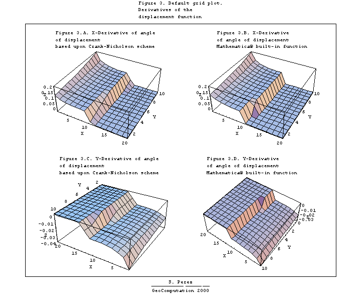
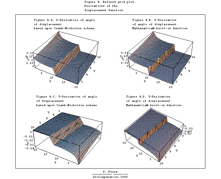
To that end the Mathematica® built-in function for derivatives allow a system-incorporated mean to get the derivatives of the displacement direction function illustrated in Figure 2, either along the X axis or along the Yaxis (Figs. 3.B and 3.D, respectively). To codify the Crank-Nicholson solution (Kreyszig, 1995), as suggested by Waltham (1989), is also a feasible task (Figs. 3.A and 3.C).
The difference between the graph of the functions is seen at the interval where there is a torsion on the displacement direction surface, as is depicted in Figures 3.A to 3.D . The Crank-Nicholson scheme produce a smooth torsion surface at the transition while the built-in function produce a sharp one for the same default interval grid size, common to all plots.
Again, the default grid size that the system uses to make plots should be refined to improve the insight in the real behavior of the functions. In Figures 4.A to 4.D the plots of the derivatives obtained by the Crank-Nicholson scheme give a steeper surface at the zone of the boundary between the displacement angle domains.
The plots for each direction of the derivatives look more similar than what is appreciated in Figure 3. Therefore, the difference between the plots seen in Figure 3 is consequence of the grid used. As a matter of fact, as the functions approaches asymptotically the real value of the derivative, the plot of both derivatives along each direction should coincide as the grid is refined.
This process involves the calculation of velocities for points outside
the grid. This is consequence of the displacement of the nodal points
as deformation evolves.
A linear interpolation function is suggested to be used to find
the velocities of the displaced points.
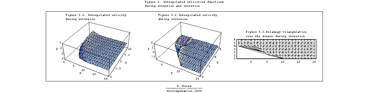
To tackle this is necessary to find a way to make interpolation over an scatter, non-regularly spaced distribution of points.
To the authors knowledge only the ExtendedGraphics package developed by Wickam-Jones (1994) provides an answer to this situation. The TriangularInterpolate function from this package does allow to make linear interpolation of scattered distribution of points. It can be downloaded from the Mathematica® website.
The graph of the function applied to the extension and inversion velocity data is seen in Figures 5.1 and 5.2, respectively. The Figure 5.3 displays the default delaunay triangulation, in plan view, that is (inferred) to be used by the TriangularInterpolate function.
As it is appreciated in Figure 5.2, the plot of the dataset obtained from the TriangularInterpolate function (made using the built-in function ListSurfacePlot3D) assumes a triangulation scheme that interpolates points from the listric fault across the upper ramp-detachment level, and leaves an open, non-interpolated narrow area between the ordinates 4 and 3.
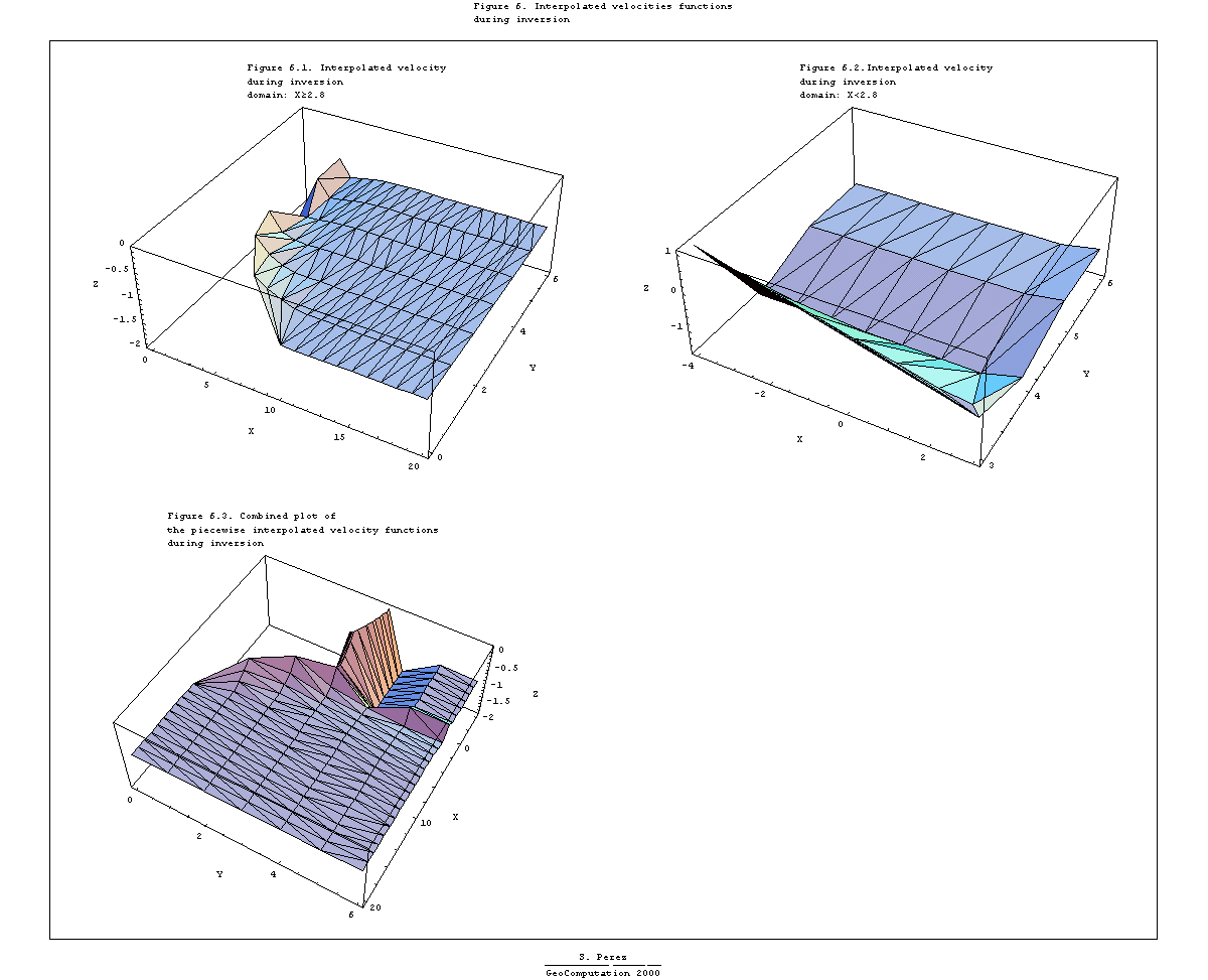
But one thing seems to be the triangulation followed by the display of the function (Figure 5.2) an another the triangulation followed by the TriangularInterpolate(Figure 5.3) function to make the interpolation. Since both are not necessarily the same, one way to tackle this inconvenient is to split the interpolation in two zones where the TriangularInterpolate function and ListSurfacePlot3D operate according to the real boundary domain of the model (Figs. 6.1, 6.2 and 6.3).
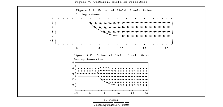
At this stage, the rate and direction of displacement for a particle at any point of the hanging wall during extension or inversion can be displayed using the function for visualising vectorial fields (Figs. 7.1 and 7.2):
Nevertheless, the basic algorithm programmed does not include neither the difussion equation nor the compaction due to burial (Waltham, 1992). Hence is an ideal simulation of syn-tectonic sedimentation below water level at shallow burial depths.
During inversion is feasible to analyse the dynamics of features like the evolution of the position of the null point, the development of the inversion anticline coupled with the fault-related fold and the deformation of the pre and syn-inversion sequences (last frames of the animation).
One of the features that the finite-difference model designed by D.
Waltham awaits for enhancement deals with 3D out-of-plane movements and
deformation of the hanging wall, like happens during transpression or transtension
in strike-slip settings.
The resources provided by high level systems of doing mathematics by
computing seems promising to supply tools that could pave over the
way toward developments in such topics.
Respect to Mathematica® itself, two comments are made.
First, the brief inspection of the outcomes for the derivatives of the
angle of displacement direction indicates that care must be taken to crosscheck
the effects on the calculations due to the default interval sample that
the system uses when operates over functions.
The desired level of accuracy can be obtained changing the default
settings accordingly.
Second, the system is under active development by a Research Group and hopefully high standard built-in tools will be available soon to tackle efficiently all the spectra of specific problems that arise in the process of interpolation of non-uniformly datasets, usually found to develop finite element models, either linear or non-linear.
But by now the ExtendedGraphics package is unsupported and seems to have inconvenient handling figures with the default format from lists, so undetermined values could be returned from points within the interpolated area during the run of the loops. Step-by-step calculations are then needed to make the interpolations and the process is time consuming.
The default triangulation process of the TriangularInterpolate function
is difficult to visualice for complex shapes usually found at the
boundaries of geological models, but not to say finite element domains
in general. One standing question is whether or not ListSurfacePlot3D makes
the same triangulation as the TriangularInterpolate function. Splitting
the data to create piecewise interpolating functions is a solution
to avoid doubtful results, but hopefully a more advanced version of
ListSurfacePlot3D will be available soon to control visually the boundaries
where the TriangularInterpolate function or an equivalent one
is needed to be adjusted.
2. Regarding the resources required from the system for linear finite-element programming, a wise and critical attitude should be maintained over what is Mathematica® doing. Specifically to avoid a "black box" usage of the tools supplied by Mathematica® it is recommended that:
2.1. When the graphical outcome of functions are analysed, care must be taken to distinguish between what is consequence of the mathematical properties of the function itself and what is consequence of interpolation over the grid interval size applied to its graphical display.
2.2.When complex boundary shapes are involved in the modelling it is
recommended to crosscheck the default triangulation process that operates
for ListSurfacePlot3D if this function is applied to visualise values given
by the function TriangularInterpolate. The default triangulation process
that operates for TriangularInterpolate itself should be controlled
as well.
The application of those built-in functions over domains splitted
off non-complex boundaries would be a confident way to use
them.
The author wish to give thanks to the following persons:
To Dr. Dave Waltham, by his valuable comments and suggestions.
To Cipriano Cruz, now at the Coordinacion Academica of the U.C.V., by
the benefits the author owe to his standard of excellence in undergraduate
calculus teaching.