GeoVISTA Studio: a geocomputational workbench

Mark Gahegan, Masahiro Takatsuka, Mike Wheeler and Frank Hardisty

GeoVISTA Center, Department of Geography, 302, Walker Building, The Pennsylvania State University, University Park, PA 16802, USA.

Email: mark@geog.psu.edu URL: http://www.geog.psu.edu/~geovista/

Abstract

One barrier to the uptake of Geocomputation is that, unlike GIS, it has no system or toolbox that provides easy access to useful functionality. This paper describes an experimental environment, GeoVISTA Studio, that attempts to address this shortcoming. Studio is a Java-based, visual programming environment that allows for the rapid, programming free development of complex data exploration and knowledge construction applications to support geographic analysis. It achieves this by leveraging advances in geocomputation, software engineering, visualisation and machine learning.

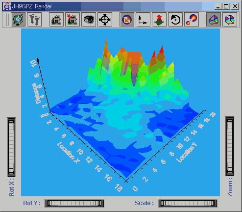
At the time of writing, Studio contains full 3D rendering capability and has the following functionality: interactive parallel coordinate plots, visual classifier, sophisticated colour selection (including Munsell colour-space), spreadsheet, statistics package, self-organising map (SOM) and learning vector quantisation.

Through examples of Studio at work, this paper demonstrates the roles that geocomputation and visualization can play throughout the scientific cycle of knowledge creation, emphasising their supportive and mutually beneficial relationship. A brief overview of the design of Studio is also given. Results are presented to show practical benefits of a combined visual and geocomputational approach to analysing and understanding complex geospatial datasets.

Keywords: geocomputation, visualisation, knowledge discovery, classification, inference.

1. Introduction

Geocomputation encompasses a wide range of different tools and techniques, including data mining, knowledge construction, simulation and visualization, all operating within the geographical realm. These activities take place along the entire extent of the scientific process, often beginning with abductive tasks such as hypothesis formation and knowledge construction, through inductive tasks such as classification and learning from examples and ending with deductive systems that build prescriptive models (that are common in spatial analysis and GIS). However, unlike GIS, there is no standard package or system that currently supplies these different types of functionality as an integrated whole, instead users must resort to a set of disparate (and often clumsy) programs that are difficult to connect together operationally. This is a serious problem, and probably the biggest barrier to the uptake of geocomputational methods currently.

Making such methods freely available and able to work in harmony is a difficult task involving conceptual challenges associated with knowledge construction as well as practical difficulties in a software engineering sense. One possible solution is to build a software environment that can hide some of the engineering, metadata and conceptual problems from the user, whilst at the same time offering extensibility and the ability to customise. GeoVISTA Studio is such an environment, offering programming-free software development for a combination of geocomputation and geographic visualization activities. Studio employs a visual programming interface, allowing users to quickly assemble their own applications using a data-flow paradigm from a library of functionality implemented as JavaBeans™ (JavaBean is a trademark of Sun Microsystems, Inc., 901 San Antonio Road, Palo Alto, CA 94303 USA.)

After the following motivation section, the roles that geocomputation and visualization can play throughout the scientific cycle are described (Section 2), emphasising their supportive and mutually beneficial relationship. Section 3 then examines some of the alternative methods by which knowledge is constructed, and shows how they might be integrated conceptually. Following this, an overview of the architecture of Studio is given. (Section 4). Example results from Studio are then presented in Section 5 to show practical benefits of a combined visual and geocomputational approach to analysing and understanding complex geospatial datasets.

1.1 Reasons for building Studio

It is worth noting at the outset that building tools to support knowledge construction and other geocomputational activities is not straightforward because little is known yet about how these activities might be formalised by a machine, or even how they might interact effectively. So, the building of a geocomputational environment is at this stage somewhat speculative, it is not possible to produce a design specification based on functionality, as is common within the GIS industry. Bearing that in mind, the following list of points acts as both motivating factors and design goals.

Humans engage in many different forms of reasoning (Section 3 takes this up further) when tackling a scientific problem, yet current GIS address only one explicitly, namely deduction, and provide only ad-hoc support for others. New types of co-ordinated functionality are needed to generate the categories, hypotheses, relationships and objects that GIS employ.
We do not know yet how best to support these knowledge and hypotheses construction activities. By assembling together a range of learning, knowledge discovery and visualisation tools in the same environment we can more easily investigate the kinds of tools, linkages, controls and meta data that prove to be effective in an operational setting. In doing so we hope to learn how to make this kind of functionality interoperable in the future.
Stronger links between visualisation and geographical analysis are required. GIS are getting better at visualising data, but are still largely tied in to the cartographic paradigm, so lack the flexibility and functionality required to support visualization targeted at knowledge construction. Furthermore, some geographic simulation models are becoming so complex that it is imperative to have visual means of tracking and steering their behaviour as they execute (e.g. coupled atmosphere and ocean climate models, Hibbert et al., 1996).
It is very difficult to exchange geographical models with other researchers. Although standards for exchanging data are now quite advanced, we have perhaps have lost sight of the fact that our data is only useful with appropriate analytical models (Goodchild 2000), and do not yet know how to make these interoperable. Studio provides both an environment in which complex functionality can be linked together into models, and a simple method to 'wrap up' the assembled functionality into an application (a JavaBean) that can be easily disseminated. Furthermore, using Bean technology, it is straightforward to extend these models or couple them to additional methods (Section 4 gives more detail).
By combining visual and geocomputational approaches within the same environment, many benefits are realisable; three cases follow. Firstly, a visual interface allows abductive knowledge discovery agents to report their findings within a visual domain, thus drawing the expert's attention to potentially significant patterns within highly multivariate data spaces. Secondly, inductive learning agents can be trained in these visual data spaces from anomalies and structures recognised by human experts. Thirdly, visualization allows the behaviour of machine learning tools to be monitored during training or configuration as a form of audit and control to ensure correct functioning (e.g. visualization of hyperplane movement in neural networks). Section 5 provides some practical examples.

1.2 Studio Capabilities

At the time of writing, Studio has the following functionality:

full 3D rendering capability including frame-by-frame animation, as is available in Viz5D (Hibbert et al., 1996) but with the addition of full control over all visual variables during 'playback';
interactive parallel coordinate plots, for dynamically visualising the relationships between many attributes (Inselberg, 1997; Edsall, 1999);
a visual classifier, to convert continuous variables into mapable discrete colour ranges (Slocum, 1999: Chapter 4), including manual and Jenks Optimal methods (Jenks, 1977);
sophisticated colour selection, including RGB and Munsell colour-spaces (Slocum, 1999: Chapter 5);
a spreadsheet, for keeping track of numerical values and for co-ordinating data selection activities with other components;
a statistics package, to provide descriptive statistics on both samples and populations, including some rudimentary spatial statistics and a range of analysis and classification methods including: k-means clustering, ISODATA and maximum likelihood (Dunteman, 1984);
self-organising map (SOM) and learning vector quantisation (LVQ) neural networks (Kohonen, 1995) for classification, pattern analysis and machine learning in complex feature spaces.

2. The Spectrum of Science

Our efforts to understand and model the world around us take many forms (Mark et al., 1999). Even when a scientific perspective is specifically adopted, there is no single universal standpoint or origin from which to begin; the creation or uncovering of knowledge occurs at many levels and starts in many places. What we see in GIS, for example, is often a well-ordered world, comprised of discrete objects drawn from crisp categories, and associated together with a small and precise set of logical relationships. Analysis in GIS often starts with these objects, categories and relationships being accepted as 'given', and proceeds to use them as part of some deterministic model. The fact that GIS has proved itself to be beneficial in a number of organisations and practical settings attests to the usefulness of these starting assumptions. However, we do well to remember that they are assumptions, nothing more. GIS are successful precisely because prior activities such as fieldwork and data interpretation produced the objects, categories and relationships used, from less abstract sources of information.

The idea, often implicit in GIS, that objects and categories have some sort of 'natural' existence and order just waiting to be 'uncovered', is a very old one, cropping up in the teachings of Aristotle. It has been justifiably claimed that humans need categories to function (Lakoff, 1987) and it appears that GIS do too! However, anyone who has worked with landcover classification, geological mapping or eco-regions, for example, will well understand the difficulty in creating classes in the first instance, not to mention the problem of communicating them effectively to others. Conversely, those who have needed to use such classes, but who did not play a part in creating them, will be acutely aware of the frustration of never being fully certain of what a class is supposed to represent. To make matters worse, often the only clue to the true identity of a derived class is in the name or label it is given and possibly a short description in an annotated legend.

This description highlights a number of problems:

Constructing categories, objects and relationships requires different tools to the ones available in GIS.
Geospatial information is often constructed in a different system to the one within which it is applied, and increasingly not by the people who will be the end users.
There is often a good deal of information loss when data are moved from the system that created it to one that will apply it.
This lost detail may later be critical in understanding or correctly applying some created object.

Geocomputation activities span this full range of knowledge construction, and indeed are often associated with activities external to GIS because they are creating information for a GIS to use.

3. Knowledge Construction

Focussing just on categories, this section describes different ways in which categories can be formed, and some of the tools that might support their construction. The structure and internal form of categories has long been debated within philosophy and psychology (e.g. Peirce, 1891; Rosch, 1973; Baker, 1999) and has more recently received interest from the machine learning community as algorithms are designed to automatically construct and recognise (label) categories (e.g. Mitchell, 1997; Luger & Stubblefield, 1998; Sowa, 1999). This interest has stemmed from the real need to extract information from large and complex datasets and reduce large data volumes and complexities into some manageable form, for example by using data mining or classification (Piatetsky-Shapiro et al., 1996; Koperski et al., 1999; Landgrebe, 1999).

3.1 Defining categories

We now briefly address the issue of how categories might be defined in order to understand better how computational methods might help. A number of different mechanisms have been proposed by which a category might be defined, based on cognitive studies of humans. A comprehensive overview is given by MacEachren (1995: Chapter 4). The following are three of the most obvious:

Typical examples, not necessarily real (e.g. Crocodile Dundee as a typical Australian). Typical (but imaginary) examples are sometimes included in map legends, in the interests of clarity.
Exemplars or best examples (e.g. Rock groups: the Beatles, the Stones). These are defining examples that demonstrate the range or scope of a category, and about which other members may cluster.
By some attributes or properties and their relationships (e.g. a hot day is one where the temperature exceeds 25° C). Most machine learning tools classify data using attributes only so their categories are of this form.

The process of constructing a category in the absence of prior knowledge is often associated with the inferential mode called abduction. Taking some examples of a category and then producing a generalised description that can be used, say for classification, uses an inductive mode of inference. More on inferential mechanisms follows to help motivate the need for new tools with which to perform geographical analysis. A full description of inference in the earth sciences is given by Baker, 1999).

Deduction

A deductive tool behaves in a deterministic manner. It is not able to adapt to the particularities of any given dataset so its outcome is defined purely in terms of methods or rules that are pre-defined. Inductive and abductive tools will produce different results if the dataset is changed because they rely on the data to help structure the outcome (see below). In the example above, defining a day as 'hot' if the temperature exceeds 25° C, is deductive. The category would remain the same even if, in reality, most days have a temperature above 30° C. Deduction is most useful where a system is clearly understood, as in category type 3 above.

Induction

With induction, characteristics in the specific data under consideration help to shape the definition of a category. To continue with the above example we might choose some sample days that we would term as 'hot' (i.e. the concept of 'hot' is pre-defined by examples) and then construct a general category from the attributes of the sample. In doing so we might find that the concept of 'hot' varies with humidity as well as heat, or varies with place (e.g. from the UK to Australia), or varies with time (from summer to winter). Induction is very useful if the concept to be defined is complex, the dataset is complex or we are uncertain how to define the concept deterministically, but are confident in our ability to point to examples (category types 1 and 2 above). For precisely these reasons, inductively-based classifiers are now becoming common in remote sensing applications, especially when dealing with hyperspectral or multitemporal data (Benediktsson et al., 1990; Foody et al., 1995; German & Gahegan, 1996). They may well also become a crucial tool for understanding the large geospatial databases now being created for socio-demographic and epidemiological applications, simply because they are able to scale up to very large attribute spaces more readily than conventional deductive approaches (Gahegan, 2000). Field scientists often perform induction when they are presented with a number of examples of some phenomena from which they must form a mental model of a category, an example of the second way by which categories might be defined given above.

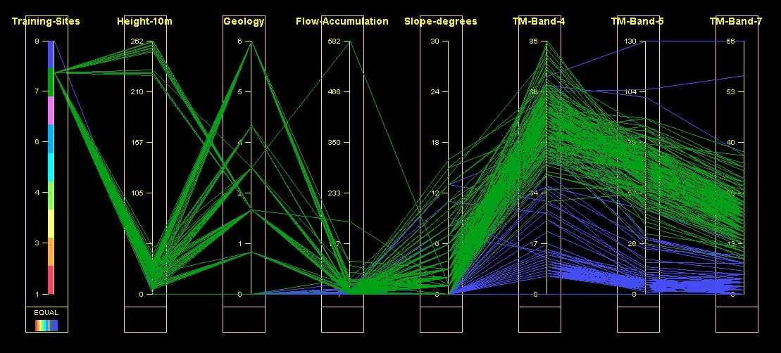
Figure 1. Visual analysis of class separability using a Parallel Coordinate Plot. See text for details. Figure 1 shows part of an inductive exercise. The categories in this case have been imposed upon the data (the left-most axis) and two of them, water (blue strings) and cleared land (green strings) are explored for potential class separation problems with during classification. In this case the two classes separate well on many of the available attributes, but note the presence of some strange outliers, especially blue strings with very high values for Landsat TM-Band-5 and TM-Band-7. These are likely to be erroneous and should probably be removed prior to classification (see later).

Abduction

Abduction is the inferential mechanism used to generate categories in the first place. In the Earth sciences, abduction is usually driven by observations (data) and expertise working together. True abduction must propose a categorisation and simultaneously give a hypothesis by which the category can be recognised or defined. It is our own adeptness with abductive reasoning that makes humans good Earth scientists. For example, when a field geologist is logging an area, the categories to be used may not be clear or fixed at the outset and new categories might need to be created. Furthermore, simple labels are not the only outcome, the categorisation produced has as its hypothesis an evolutionary geological model explaining how each category might have come to be. Categories may be based on form, structure, mechanical and chemical properties and reliance on any of these properties may differ from category to category. They may well also reflect the education, biases and experience of the geologist in question (see Brodaric et al., also in this volume). In computational data mining, unsupervised classification or clustering is often used to identify candidate categories, with the algorithm that separates the classes (class definitions) provided as the hypothesis. In contrast to the geology example, this is perhaps a weaker form of abduction because the hypothesis produced only relates to the attribute values in the data, and not to any additional (externally held) knowledge.

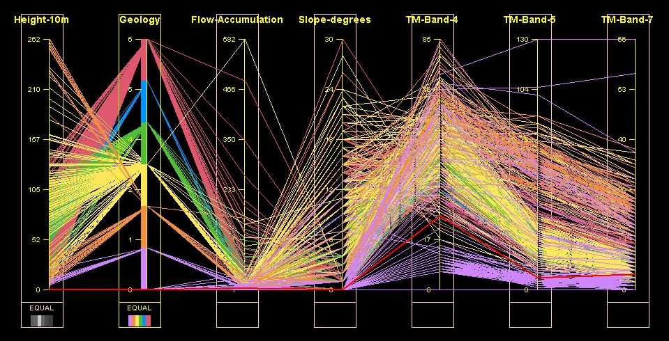
Figure 2. Using a parallel coordinate plot to search for possible classes in unstructured data. An example of the search for possible classes is shown in Figure 2. In this example, the target landcover categories are undefined and the user is exploring the clustering in the data that is characteristic of the 'Geology' attribute. There appears to be some kind of partial relationship between the remote sensing channels and this attribute, as evidenced by large swaths of yellow and purple strings concentrating in the TM-Band-4 and TM-Band-5 axes.

3.2 Combining inferential tools and techniques

Having defined these generic types of inference, it should be clear that geographers are in fact quite skilled in utilising all three, often in combination and with no pre-defined methodological structure. That is to say, there is no single mechanism by which these types of inference should be combined; the task of building a 'system' for knowledge construction is itself non-deterministic.

Figure 3 shows one possible arrangement for deriving categories from data, involving iteration between abduction and induction. Visualisation can play a key role in a number of these stages: in presenting a visual overview of the data so that categories might be hypothesised, in evaluating individual examples with respect to their 'representativeness', in portraying the boundaries between categories (e.g. in feature space) and in showing the results of applying the new knowledge to structure the data (Lee & Ong, 1996; Keim & Kriegel, 1996; MacEachren et al., 1999).

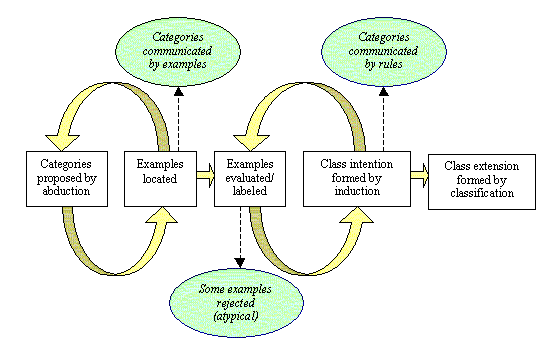
Figure 3. One possible scenario for the iterative construction of knowledge, involving first abductive then inductive reasoning.

The results (Section 4) show examples of knowledge construction and analysis using a variety of inferential tools and visualization methods, working in combination.

4. The Design of Studio

In order to carry out the sophisticated data analysis tasks outlined above, a system has to bring together the various kinds of geocomputational tools and techniques mentioned in Section 1.2. At its heart Studio has a component-oriented software building system (called "builder") that employs a visual programming environment to connect program components together into useful applications (see Figure 4).

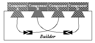
Figure 4. A builder constructs an application by connecting program components. The builder allows different components, each offering pieces of the required functionality, to communicate freely with each other. However, the nature of these connections, i.e. what should be connected and how, is not clear at the outset (as described in Section 3.2). Consequently, the system needs also to provide an experimental environment to test and discover how components should be connected to maximise the effectiveness of constructing knowledge or otherwise analysing geographical data. To meet these and other needs, the builder was designed to address the following points: "Open Standards", "Cross Platform Support", and "Integration and Scalability".

4.1 Open Standards

A builder has to accommodate components (tools) developed by different parties. In order to handle this multi-developer problem, component design must adhere to well-established standards. Studio employs Java as the system programming language and so uses JavaBean technology to construct tools. All visualization, geocomputation, machine leaning and other components are implemented in the form of JavaBeans. The JavaBean specification defines a set of standardised, component, Application Programming Interfaces (APIs) for the Java platform. As long as a component is built according to this specification, it can be incorporated into any JavaBean capable builders as shown in Figure 5.

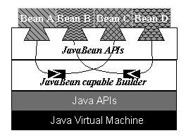
Figure 5. The builder integrates JavaBeans by using JavaBean APIs. For the developers of components, this provides a straightforward mechanism to ensure their components can be employed by many users (see Figure 6), and is therefore extremely useful at increasing productivity in a postgraduate laboratory setting! In other words, the end users can employ a wide variety of JavaBean components developed by various suppliers. In using a JavaBean component, a JavaBean capable builder automatically finds out a syntactic description of its functionalities and input/output methods as described below in Section 4.3.

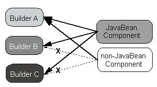
Figure 6. A JavaBean is accepted in any JavaBean capable Builders. A non-JavaBean component is only usable in a propriety builder.

4.2 Cross Platform Support

Studio is designed to run on various operating systems (Solaris, Windows, Linux, IRIX, etc.) and hardware architectures (Intel, SPARC, MIPS, etc.). Since Studio itself is written in pure Java, Studio and its JavaBean components will run on any operating system and hardware combination as long as a Java Virtual Machine is available. (To check on currently supported platforms, refer to http://java.sun.com/cgi-bin/java-ports.cgi.) Moreover, Java's network capability allows a user to build network-aware systems for heterogeneous hardware and operating system environments. For instance, imagine a situation where two JavaBeans, A and B, are processing a task together. If component B is carrying out a computationally heavy task, a user might want to execute this component on a more powerful machine. If both A and B implement network functions, they can still communicate with each other as if they were executing on the same machine (see Figure 7(a)). Even if both components do not have network capabilities, a user can achieve the same result by connecting them using network capable JavaBean components (see Figure 7(b)).

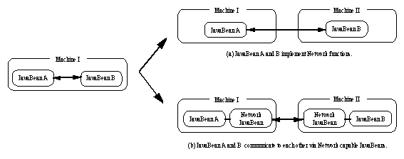
Figure 7. Using Java's network capability, JavaBeanson different (hardware and software) platforms can seamlessly communicate.

4.3 Integration and Scalability

Studio, as a builder, must be able to integrate various kinds of components from a multitude of sources. Studio provides a basic set of JavaBean components, most of which are independently executable. A user can combine these components to construct useful visualization, geocomputational, and machine learning systems. However, solutions to a specific problem might be difficult to build using only the pre-supplied components; a user might wish to add in locally-produced components, or might obtain components from some other source (Due to the popularity of Java, there are many useful JavaBeans available already on the Internet). In all cases, Studio has to provide a mechanism to integrate any JavaBean component, regardless of its source.

In order to meet these requirements for a JavaBean capable builder, Studio utilises Java's introspection functions. With these functions, Studio is able to find out what kinds of input and output are available as well as all the customisable properties of a bean when it is dynamically added to Studio. A JavaBean sometimes supplies its own tool to customise itself. Even in this case, Studio is able to incorporate this special customising tool by using interfaces defined in the JavaBean specification. With these features, Studio does not need any prior knowledge of a new JavaBean in order to integrate it into a program developed under Studio. This is a clear advantage over older mechanisms involving recompilation and linking, such as used in third generation computing languages.

Studio utilises Java's event model in order to let a user connect JavaBean components together. When something of interest happens within a JavaBean, the bean notifies other components by sending an event object (like sending a message). When a user connects two JavaBeans with a mouse dragging action an event adapter object, which is invisible to a user, is created and is registered with an event source JavaBean as an event listener object. When the event adapter detects that something interesting happens it will call an appropriate method on the target JavaBean component.

Studio is also capable of 'wrapping' a whole connected graph of JavaBean components into another single JavaBean. This allows a user to gradually build up large scale and complex applications by constructing from small and less complex components. Moreover, any JavaBeans constructed at each stage of this gradual development can be shared or distributed among colleagues since they are independent working program components.

5. Experiments using Studio

Two sample experiments are shown here, both aimed at investigating the structure inherent in a large and complex dataset.

The first shows the co-ordinated application of: 1) a spreadsheet, showing numerical values for individual data records; 2) an interactive Parallel Coordinate Plot (PCP), depicting each record as a single 'string'; 3) a Visual Classifier (VC), to interactively impose a categorisation on the data; 4) an unsupervised k-means classifier. Using the Studio environment described above these components are connected together as shown in Figure 8. Other ancillary beans to read in and visualise data also appear in the figure.

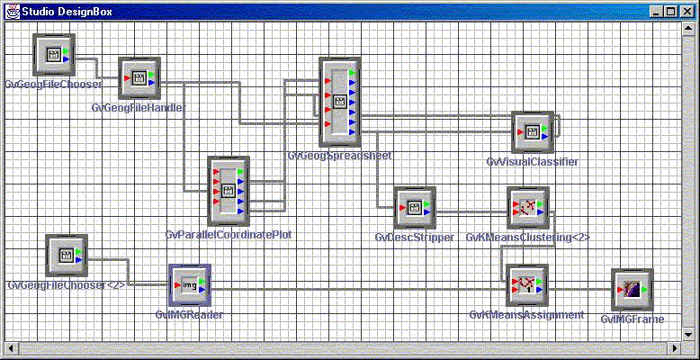
Figure 8. Design Box from Studio showing components connected for data exploration leading to classification. See text for details. Connections show the flow of data and co-ordination of activities between the beans

The spreadsheet, PCP and VC can be used together to help explore an unfamiliar dataset and lead to the configuration of a successful classification. The PCP and spreadsheet allow the user to explore the data for outliers, errors or missing values that can then be removed or corrected prior to classification, since their inclusion will likely lead to problems. The VC and PCP allow the user to experiment with different class structures by changing the colours used for each of the strings, according to some chosen attribute value. This helps the user to hypothesise structure or relationships within the data (the beginnings of abduction) and also to select an appropriate value for k, the number of classes to be used in classification. To aid co-ordination, the components possess a degree of interaction. 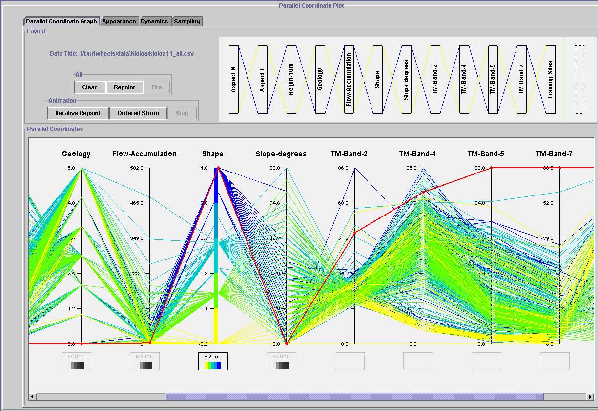For example, clicking on a string in the PCP will select the appropriate row in the spreadsheet, and vice versa. Figure 9 shows an outlier in the PCP (in red) that has been visually identified. Selecting it (with the pointing device) automatically highlights the offending record in the spreadsheet (Figure 10). It can then be deleted if required. Other selection behaviours are also co-ordinated, for example selecting an axis in the PCP will highlight a column in the spreadsheet, and change the focus of the VC, and so forth. The selection of appropriate class breaks for visual display, using the VC is shown in Figure 11. The data, minus any problematic examples that are removed via the PCP or spreadsheet, are then passed to the k-means classifier which then computes k centroids to represent data classes. These centroids are then used to generalise to the entire dataset to form the classified image shown in Figure 12, an inductive step. Without removal of the problematic data, the final mapped result can be markedly different to that shown.

Figure 9. An interactive PCP used to study suitability of a training sample. An outlier is shown in red, and this can be deleted if required. Strings are grouped into five classes from a visual classification on the 'Shape' attribute.

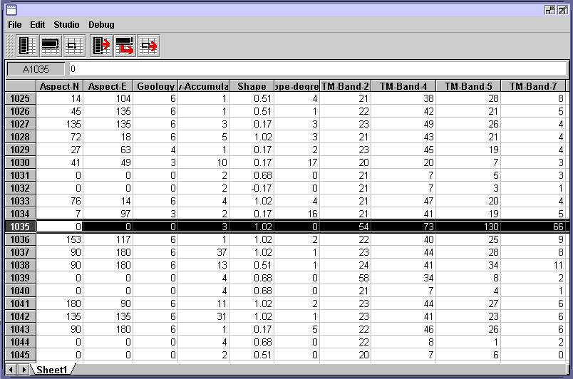
Figure 10. The spreadsheet, showing part of the training data and automatically selecting the troublesome example highlighted in the previous figure.

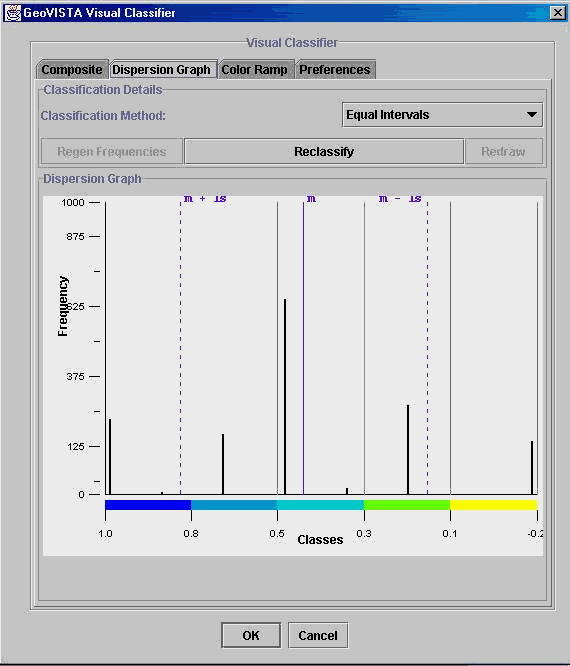
Figure 11. The Visual Classifier (VC) used to assign data ranges to the five colours shown in the parallel Coordinate Plot above.

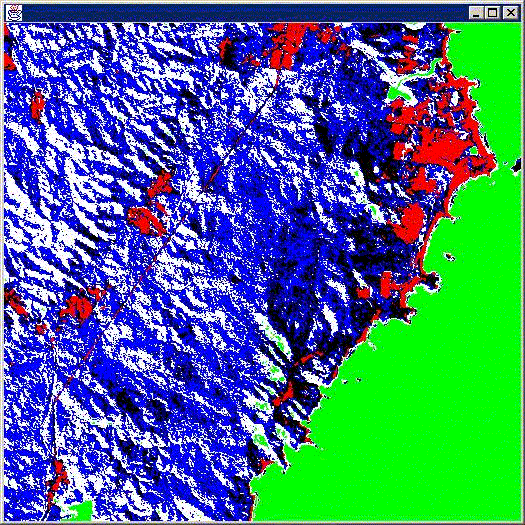
Figure 12. Results of running a k-means classifier on the cleaned up dataset shown above. The green class represents water, red is cleared land, blue, black and white represent a mixture of forest vegetation types.

The components described above are shown, as they appear in Studio operationally, in Figure 13.

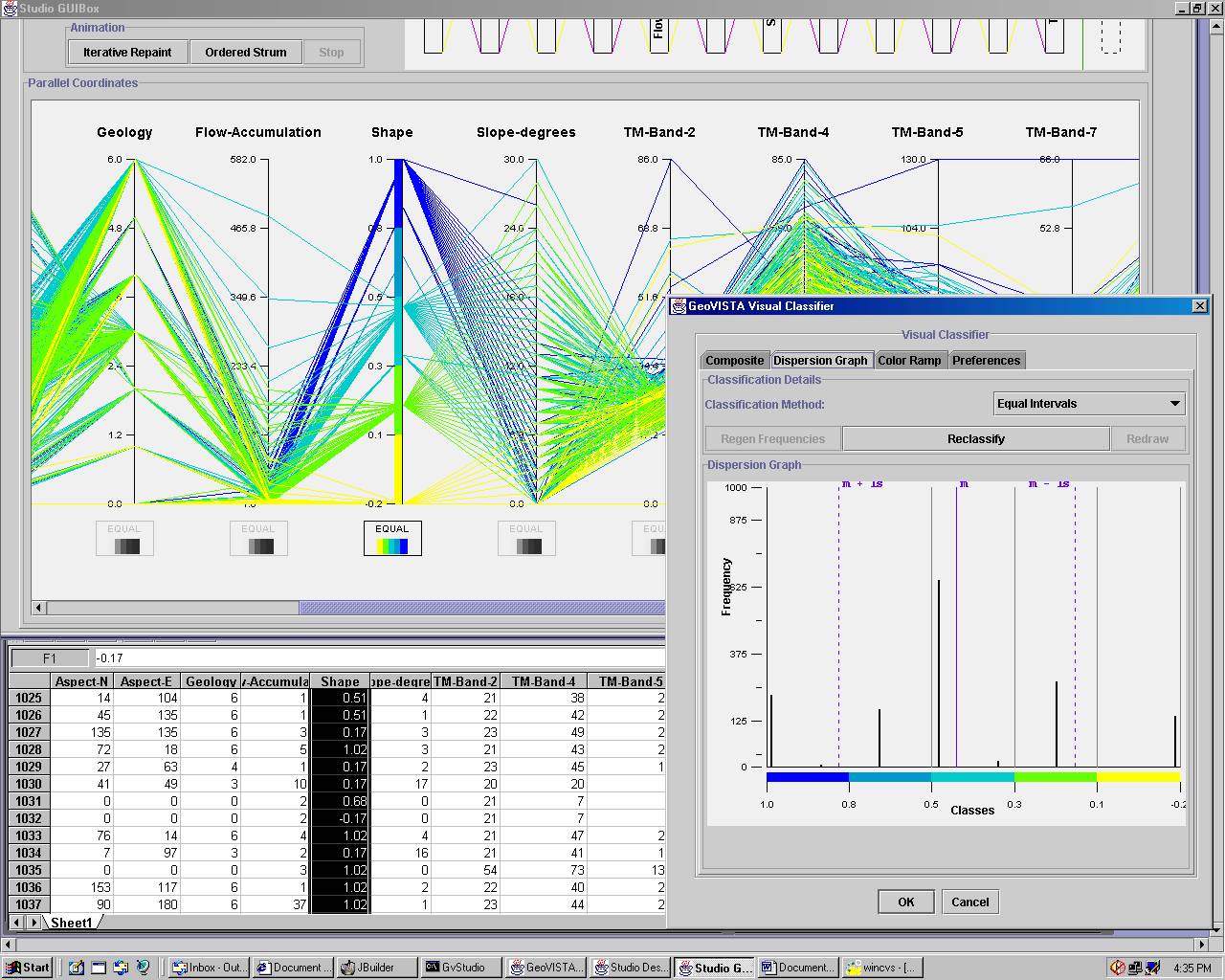
Figure 13. A screen snapshot from Studio of the classification exercise described above.

If a more sophisticated classifier is used, such as Kohonen's Self Organising Map (Gahegan & Takatsuka, 1999), then one associated problem has been the difficulty in understanding the inner workings of the classifier, thus lowering our confidence in the outcome it produces and oftentimes leading to exhaustive testing as a substitute. However, Studio allows us to simply connect the state of the hidden layer of neurons at each timestep (a 2D array of distance measures forming a surface) to the 3D renderer so we can observe the classifier training in real time and ensure that it does indeed converge to a reasonable solution. Figure 14 shows four timesteps from the convergence of such a neural network and indicate a stable progression towards the final outcome (a good sign).

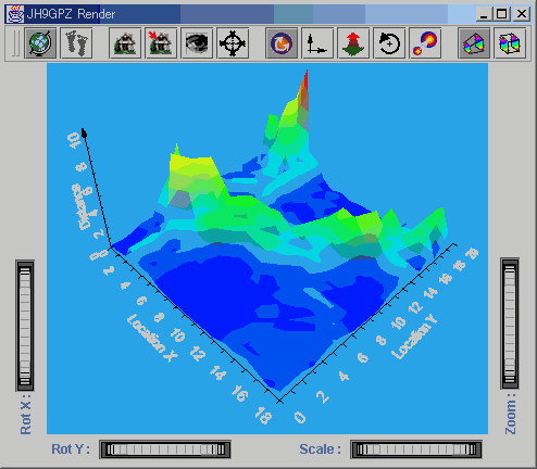
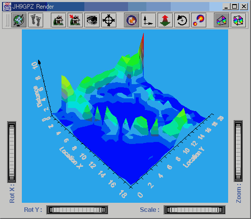
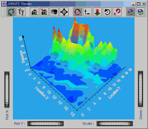
Figure 14. Images from the inside of the Self Organising Map. The 3D rendering shows distance between neighbouring neurons in feature space. Distance is normalised on the z axis from 0 - 10, with colour and height both visually encoding this distance. The images show clean convergence of the network at iterations 100 (top left), 300 (top right), 600 (bottom left) and 900 (bottom right).
The above applications were created without resource to conventional programming, but instead by connecting together a series of independently created components. These components form the backbone of Studio and obviously have been designed to integrate effectively. However, other geocomputational tools can be added into the mix with ease.

6. Conclusions and Future Work

With the continued development of advanced computational and visualisation methods, coupled with a greater understanding of how these can be applied to geographical problems and accompanied by breakthroughs in software engineering we are entering an exciting era of new possibilities for geographical analysis. Studio represents one approach for taking advantage of these possibilities and is a serious attempt to address the fundamental problems associated with knowledge discovery, exploratory analysis, classification and object creation as they relate to geography. It is perhaps too early to say whether the design of Studio facilitates these tasks effectively, but our own experience in developing the applications described above shows a promising gain in efficiency over traditional programming methods, and a much greater degree of integration and co-ordination among the component pieces, fostering easier exploration and better understanding of both tools and data.

With the visual programming environment now completed, future Studio development effort will focus on specific tools for geographic visualisation and analysis. Our current plans include interactive scatterplots, Bayesian knowledge discovery agents, and metadata (including semantic histories) to allow us to study and communicate the formation of geographic objects in greater detail. Further information about Studio, including sample images and downloadable applications and data are available from http://www.geovista.psu.edu/studio/. Future developments will also be posted to this site.

References

Baker, V. R. (1999). Geosemiosis. GSA Bulletin, May 1999, 111(5), 633-645.

Benediktsson, J. A., Swain, P. H. and Ersoy, O. K. (1990). Neural network approaches versus statistical methods in classification of multisource remote sensing data. IEEE Transactions on Geoscience and Remote Sensing, 28(4), 540-551.

Dunteman, G. H. (1984). Introduction to multivariate analysis. Sage Publications, New York, USA.

Edsall, R. M (1999). The dynamic parallel coordinate plot: visualizing multivariate geographic data. Proc. 19th International Cartographic Association Conference, Ottawa, May 1999. URL: http://www.geog.psu.edu/~edsall/JSM99/paper.htm.

Foody, G. M., McCulloch, M. B. and Yates, W. B. (1995). Classification of remotely sensed data by an artificial neural network: issues relating to training data characteristics. Photogrammetric Engineering and Remote Sensing, 61(4), 391-401.

Gahegan, M. (2000). On the application of inductive machine learning tools to geographical analysis. Geographical Analysis, 32(2), 113-139.

Gahegan, M. and Takatsuka, M. (1999). Dataspaces as an organizational concept for the neural classification of geographic datasets. Proc. Fourth International Conference on GeoComputation, Virginia, USA: http://www.geovista.psu.edu/geocomp/geocomp99/Gc99/011/gc_011.htm

German, G. and Gahegan, M. (1996). Neural network architectures for the classification of temporal image sequences. Computers and Geosciences, 22(9), 969-979.

Goodchild, M. F. (2000). Keynote address, Conference of the Association of American Geographers, Pittsburgh, 2000.

Hibbard, W. L., Anderson, J., Foster, I., Paul, B. E., Jacob, R., Schafer, C. and. Tyree, M. K. (1996). Exploring coupled atmosphere-ocean models using Vis5D. International Journal of Supercomputing Applications and High Performance Computing. 10(2/3), 211-222.

Inselberg, A. (1997). Multidimensional detective. Proc. IEEE conference on Visualization (Visualization '97), Los Alamitos, CA: IEEE Computer Society, pp. 100-107

Jenks, G. F. (1977). Optimal data classification for choropleth maps, Occasional paper No. 2. Lawrence, Kansas: University of Kansas, Department of Geography.

Keim, D. and Kriegel, H.-P.(1996). Visualization techniques for mining large databases: a comparison. IEEE Transactions on Knowledge and Data Engineering (Special Issue on Data Mining),

Kohonen, T. (1995). Self-Organizing Maps. Springer-Verlag, Berlin, Germany.

Koperski, K. Han, J. and Adhikary, J. (1999). Mining knowledge in geographic data. Comm. ACM (to appear). URL: http://db.cs.sfu.ca/sections/publication/kdd/kdd.html.

Lakoff, G. (1987). Women, Fire and Dangerous Things: What Categories Reveal about the Mind. Chicago: University of Chicago Press.

Landgrebe, D. (1999). Information extraction principles and methods for multispectral and hyperspectral image data. In: Information Processing for Remote Sensing (Ed. Chen, C. H.). River Edge, NJ, USA: World Scientific.

Lee, H. Y. and Ong, H. L. (1996). Visualization support for data mining. IEEE Expert Intelligent Systems and their Applications, 11(5), 69-75.

Luger, G. F. and Stubblefield, W. A (1998). Artificial Intelligence: structures and strategies for complex problem solving. Reading, MA: Addison-Wesley.

MacEachren, A. M. (1995) How Maps Work. Guilford Press, NY, USA.

MacEachren, A. M., Wachowitz, M., Edsall, R., Haug, D. and Masters, R. (1999). Constructing knowledge from multivariate spatio-temporal data: integrating geographical visualization with knowledge discovery in database methods. International Journal of Geographic Information Science, 13(4), 311-334.

Mark, D. M., Freska, C., Hirtle, S. C., Lloyd, R. and Tversky, B. (1999). Cognitive models of geographical space. International Journal of Geographic Information Science, 13(8), 747-774.

Mitchell, T. M. (1997). Machine Learning, New York, USA, McGraw Hill.

Peirce, C. S. (1891). The architecture of theories. The Monist, 1, pp. 161-176

Piatetsky-Shapiro G., U. Fayyad & P. Smith (1996). From Data Mining to Knowledge Discovery: An Overview. In: Advances in Knowledge Discovery and Data Mining, (U. Fayyad, G. Piatetsky-Shapiro, P. Smith & R. Uthurusamy, eds.), AAAI/MIT Press, pp. 1-35.

Rosch, E. (1973). Natural categories. Cognitive Psychology, 4, 328-350.

Slocum, T. A. (1999). Thematic Cartography and Visualization, Prentice Hall: New Jersey.

Sowa, J. F. (1999). Knowledge Representation: Logical, Philosophical, and Computational Foundations. Pacific Grove, CA: Brooks/Cole.