Keywords: General Regression Neural Network, Scalar Dynamics, Geocomputation, US Great Plains, Maize Production
Stating that the GRNN can be used in modeling processes operating at different scales is more than a trivial statement, especially when considering the current literature on land-use and land cover change. Scale issues are inherent in studies examining the physical and human forces driving land use and land cover changes (Fischer, Rojkov et al. 1995; Easterling 1997; Easterling and et. al. 1998; Kull 1998; TurnerII, Skole et al. 1995; Polsky and EasterlingIII 1999). A recognized need for the analysis of variables operating at multiple scales prompted the definition of scalar dynamics as defined by the Land Use/Cover Change (LUCC) program of the joint International Geosphere-Biosphere and International Human Dimensions of Global Environmental Change Programmes. Environmental problems like deforestation, soil erosion, or decreasing soil fertility result from a combination of forces. Some of these forces, such as state environmental policies, may affect large regions. Other forces, like topography, rainfall, or individual land use practices, vary locally - and it is well understood that these forces do not act alone, but in combination with each other to produce land transformations (Turner II 1995). Another type of scale issue is that of resolution, which in turn leads into data reliability or data certainty issues. Data collected at a gross scale (course resolution) is considered less reliable in aiding interpretation of events operating at fine scales (fine resolution) (Goodchild 1999). In order to effectively answer questions regarding land use/land cover changes it is necessary to account for the scale at which variables operate and to account for the scale or resolution (and thus certainty) at which the data where collected.
Given the apparent value of geocomputational techniques in aiding the interpretation of large, complex datasets, and the need to address spatial scale in modeling, this paper will discuss how the two can be integrated. Throughout the discussion the multi-scale GRNN technique will be compared to traditional OLS regression since it has been the traditional method of determining a variable's direct effects on an outcome. Three main steps will be taken to present the advantages the GRNN has over OLS regression. First, the method in which land use/land cover data are generally stored will be discussed in order to understand why such a data storage technique is not appropriate for OLS regression, but is appropriate for the GRNN. GRNN organizational structure will then be outlined. Three methods of interpreting GRNN results will also be examined in this section. Finally, strengths and weaknesses of the GRNN and possible methods of dealing with uncertainty in data are analyzed. The concluding section provides an example in which the GRNN is applied to the multi-scale analysis of corn production in the US Great Plains, making concrete the issues explored in the previous sections.
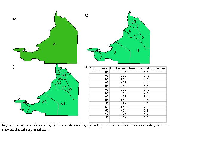
Although simplistic, the above description of multi-scale variable interaction and representation is important because that data representation causes problems when used in conjunction with OLS. When implemented in OLS regression that data structure violates a number of the assumptions of the OLS model, the most important of which is the assumption of independence of observations. The assumption of independence of observations means that knowing the value at one location does not provide a better than random possibility of knowing any other locations values based on the known value. In the above example, knowing the temperature value for one micro-region would allow someone to guess that near micro-regions had the same temperature value (Figure 1d). Furthermore, repeating macro-scale values for each recorded micro-scale value skews the calculated means, variances, and covariances of the independent (x) variables - values necessary for calculating regression coefficients (Hamilton 1992). In other words, traditional OLS regression cannot be used to analyze variables operating at multiple scales.
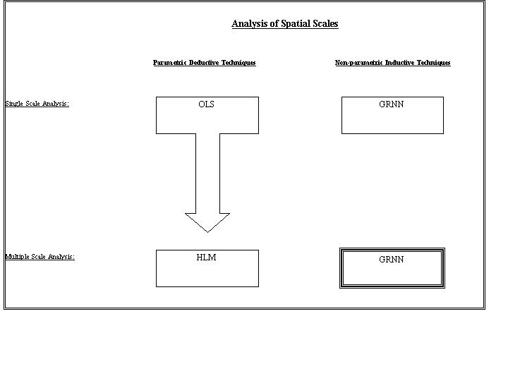
It must be stated that development efforts are underway in creating data storage methods that take into account a hierarchical data structure (Peuquet 1994; Papadias and Egenhofer 1997). Such data storage techniques are not methods of analyzing multi-scale relationships, however. Because there is a recognized need for multi-scale analysis, techniques like Hierarchical Linear Modeling (HLM) are being developed. HLM was born out of OLS regression and thus inherits most its assumptions. It does, however, effectively analyze multi-scale data by calculating separate error terms for each scale variable, (Polsky and Easterling III 1999). The GRNN, on the other hand, was developed to work under a different set of conditions than those built into OLS or HLM. The GRNN makes no assumptions about the underlying data distributions, does not require independence of observations, and requires no a priori determination of the type of function operating between variables (i.e. linear, exponential, polynomial, etc.). Until now the GRNN has not been explicitly conceptualized as a multi-scale data analysis tool (Figure 2).
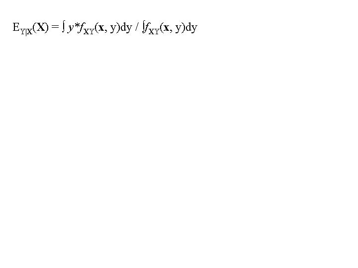
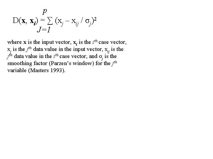
Basically there are two types of ANN's - those that predict categorical output, and those that predict continuous output. The GRNN predicts continuous outputs. Two main functions are required of GRNN nodes. Those functions are 1) to calculate the difference between all pairs of input pattern vectors, and 2) to estimate the probability density function of the input variables. Calculation of the difference between input vectors is the simple Euclidean distance between data values in attribute space. Weighing the calculated distance of any point by the probability of other points occurring in that area yields a predicted output value. With those two tasks accomplished it is a rather straightforward process of predicting the output. Equation 1
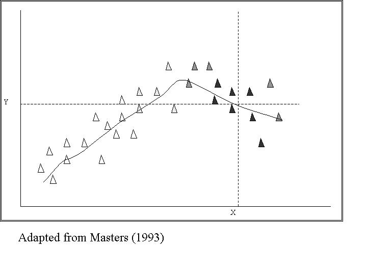
Determining the joint probability density function (pdf = fXY(x, y)dy) of the variables is the main difficulty in utilizing equation 1. Before explaining how an estimate of the joint pdf is made, a graphic example of the process accomplished by equation 1 is needed. Figure 3 is a simple bivariate example where the x-axis represents an input (independent) variable, and the y-axis represents an output (dependent) variable. Given the scatterplot displayed, one might determine a predicted y value for the new x value as shown.
The predicted y is reasonable because it is similar to the y values which have x values similar to the new x value. The colors of the scatterplot represent the similarity of the sample data points to the new x. Weights, or levels of similarity, are assigned to each point as determined by their distance from the new x, designated in the scatterplot by level of shading - dark colored points are more similar to the new x than light colored points. Little weight is given to those points that have x values very different from that of the new x value because it is not very probable that the predicted y is affected by the more distant points. Calculating all the y values for the entire range of x values would yield a curve like the one shown above. No a priori assumption was made about the shape of that curve, nor was one made about the distribution of the data. We did, however, visualize the joint probability of x and y values.
Although not difficult to understand conceptually, finding the appropriate sphere of influence for a variable can be extremely difficult. Since there is no "true" pdf with which to compare the estimated pdf another measure of the appropriate sphere of influence must be used. The appropriate sphere of influence is defined as the one that produces the smallest mean square error between the actual and predicted output values. Determination of the appropriate sphere of influence (smoothing factor, sigma) is where the "learning" takes place in the GRNN. The first smoothing factor weights assigned to each variable can take on any value. Only by varying the smoothing factor weights, based on some type of error minimization procedure, can the least square error between predicted and actual outputs be calculated. Numerous algorithms exist for optimizing sigma, ranging from steepest descent algorithms like backpropagation (which will find a local minimum) to stochastic methods like genetic algorithms (which will find a global minimum - not necessarily the global minimum, however). Although in depth discussion of optimization techniques is beyond the scope of this paper, a word about model verification is necessary. It is very possible to over train the GRNN so that is predicts extremely well the sample actual output values based on the sample input values. This occurs when the sigma weights (spheres of influence) are so small that each sample point has a very high pdf, but all pdf values between points are miniscule - the estimated pdf does not match the "true" pdf. In order to generalize about the population from which the sample was drawn, over training needs to be avoided. To accomplish this the entire sample data set is divided into two sets - a training set and a test set. The GRNN is trained and sigma is optimized on the training set. As training proceeds the error between actual and predicted values becomes smaller and smaller, and at a certain point generalization of the entire data set is compromised. In order to prevent the GRNN from over training, the test set data values are run through the GRNN after each training iteration. When over training begins, the square error of the test set begins to rise, and training stops.
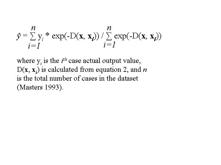
With a general understanding of pdf estimation and how that relates to equation 1, the mathematics behind Parzen's density estimator can be substituted into equation 1 to produces the following two equations.
Combining these two equations produces a predicted y in exactly the same way as was done visually in the scatterplot example (Figure 2).
When comparing GRNN results to OLS regression results, analyzing the visual relationship between predictions is also very useful. OLS regression assumes a linear relationship between data values - the GRNN does not. Although viewing a scatterplot of variable relationships prior to running OLS regression allows one to transform the variables so that they are linearly related, bias is added to the model by doing so. Likewise, other types of relationships can be modeled with regression techniques (i.e. exponential, logarithmic, polynomial), but the type of relationship must be assumed prior to running the regression. The GRNN, on the other hand, fits the relationship between variables regardless of the form of their relationship because its predictions are a result of the joint probability density function between variables. No a priori assumption about that relationship is made. Thus, plotting data points, regression lines, and GRNN lines makes possible a visual determination of which technique best fits the data. While in some cases the GRNN will not improve upon standard regression predictions, it nearly always will when the relationships are non-linear.
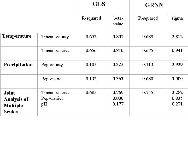
The final method of analyzing output from the GRNN is to calculate the percent of the variance in the output variable that is explained by the input variables (R-squared). R-squared in the GRNN is the same as in OLS regression analysis - it is the coefficient of multiple determination. In many cases R-squared is the final measure of which model, the GRNN or OLS regression, is the better predictor of the output. Also, multiple GRNN analyses may be run in which the same variables are used, but their scale of analysis is varied. In that situation the model whose R-squared value is highest represents the model with the most appropriate combination of scales.
It is well understood that maize production is the result of numerous biophysical constraints as well as human management of the land. Human management is subject to economic, social, and political pressures that are not taken into account here. In this simplified example the variables used to predict corn production are mean annual temperature, mean annual precipitation, and soil pH. US Agricultural Statistic Districts (ASDs), those federal government defined regions that purport to bound similarly characterized regions, form the macro-scale level of analysis. Each ASD is composed of contiguous counties, counties forming the micro-scale level of analysis. The input, or independent, variables are interpolated spatial averages for each county or ASD. The examples that follow each predict maize yield per acre at the county level, but the input variables are analyzed at both county and ASD scales.
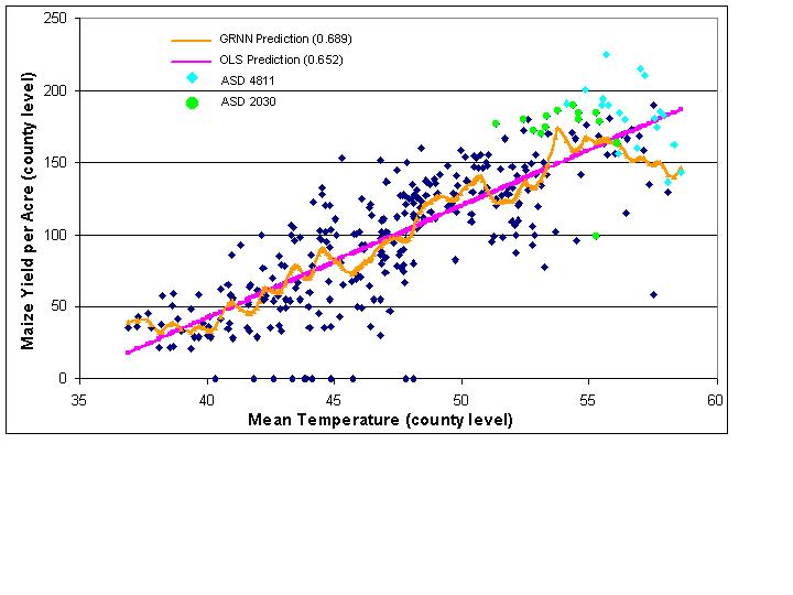
Mean annual temperature, at the county level (Figure 5), is linearly related with maize yield per acre. Both OLS and the GRNN perform similarly, visually and in terms of R-squared (Table 1). In this case, OLS regression may be used because both the input and output variables are defined at the same scale, the county, and the relationship is nearly linear. There are, however, a number of outliers (those counties that reported no corn production) that skew the line of best fit. The outliers do not as heavily influence the GRNN as they do OLS and the GRNN explains slightly more variance than OLS. At the district level (Figure 6), mean annual temperature predicts maize yield per acre similarly to the county level, with OLS explaining slightly more variance than before and the GRNN slightly less. The more interesting aspect of this graph is the arrangement of the district values along the x-axis. Since prediction of maize yield per acre is done at the county level, the number of points on the scatterplot is the same as in figure 5, but the number of x-axis values is substantially decreased. All district values are arranged in columnar form. The result is that OLS is not an appropriate technique for the analysis of this type of problem, in particular because the observations are not independent of one another. As such the line of best fit and statistical descriptors of the model cannot be trusted. Nevertheless, even with temperature values aggregated to the district level, the relationship between maize yield and mean annual temperature remains strongly linear, and both models explain a large percentage of the variance of maize production.
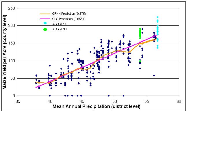
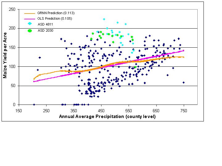
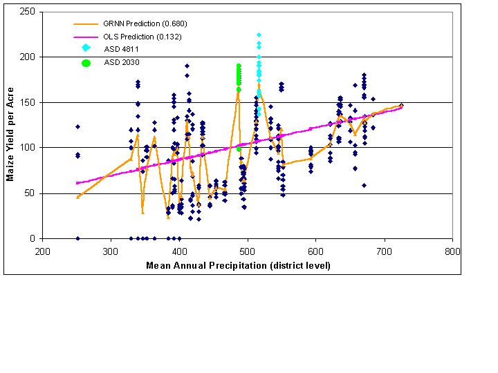
Bi-variate predictions based on mean annual precipitation are a more interesting case than those based on temperature. At the county level (Figure 7), neither the GRNN nor OLS are very good predictors of maize yield per acre (Table 1). The scatterplot reveals only a slight linear relationship, and both model types make similar predictions. One important point to notice before departing to the district level analysis is the arrangement of districts 4811 and 2030. Both districts are found in similar areas of the graph and in fact overlap. The district level analysis (Figure 8) reveals an interesting scatterplot pattern. Nearly all districts, including 4811 and 2030, are separated very well - distinguishing between districts is easily accomplished. Even before trying to model the relationships it appears that the district boundaries are effective boundaries for defining regions of similar precipitation because visually the districts are easily separated. Evidence supporting the hypothesis of effective regional delineations comes in the form of a greatly increased R-squared value for the GRNN. OLS, suffering from its limitations discussed above, improves only slightly, and it is understood that its results are skewed.
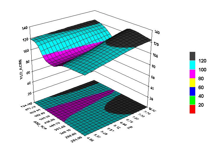
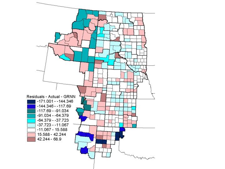
Other bi-variate relationships were analyzed in similar fashion to the two done above and from them the following joint analysis of multiple scales was devised as one that would be effective at modeling maize yield per acre. The input variables for this analysis problem are mean annual temperature at the district level, mean annual precipitation at the district level and soil pH at the county level. Naturally more complex and complete analyses would include more explanatory variables. Of the models examined, this final model is by far the best at predicting maize yield per acre, with an R-squared value of 0.755. Comparing sigma values reveals that mean annual temperature at the district level was the most important variables in predicting maize yield per acre, followed by mean annual precipitation at the district level and finally soil pH at the county level. While soil pH necessarily plays a role in maize production, examination of individual counties throughout the region reveals that nearly all the counties have pH levels suitable to maize production, which would explain why pH is less important in predicting maize yield for individual counties. As revealed by figure 9, however, it is the combination of high district temperatures and high pH that produces some of the greatest amounts of maize per acre. High pH levels in combination with low mean annual precipitation at the district level also produce high yields of corn (Figure 10). Spatially, the residual yields per acre for each county were distributed throughout the region, except for some gross over predictions in the southern and northwestern ends of the region (Figure 11). The high residuals can be explained by the fact that most of those counties did not report any corn production in the year 1995. Because the GRNN attempted to generalize over the entire region, it predicted yields in all areas, even when the actual yields for some areas were null. Overall, however, the predictions were quite accurate and outperformed the predictions of OLS regression.
Easterling, W. E. and et. al. (1998). "Spatial scales of climate information for simulating wheat and maize productivity: the case of the US Great Plains." Agricultural and Forest Meteorology 90: 51-63.
Fischer, G., V. A. Rojkov, et al. (1995). "The Role of Case Studies in Integrated Modeling at Global and National Scales." Task Force Meeting on Modeling Land-Use and Land-Cover Changes in Europe and Northern Asia March: 0-19.
Gahegan, M. (1999). What is GeoComputation?, http://www.ashville.demon.co.uk/geocomp/definition.htm. 1999.
Goodchild, M. F. (1999). "Future Directions in Geographic Information Science." Geographic Information Sciences 5(1): 1-8.
Gould, P. (1970). "Is Statistix Inferens the Geographical Name for a Wild Goose?" Economic Geography 46: 439-448.
Hamilton, L. C. (1992). Regression with Graphics: A Second Course in Applied Statistics. Belmont, California, Wadsworth, Inc.
Hewitson, B. C. and R. G. Crane, Eds. (1994). Neural Nets: Applications in Geography, Kluwer Academic Publishers.
Kull, C. A. (1998). "Leimavo Revisited: Agrarian Land-Use Change in the Highlands of Madagascar." Professional Geographer 50(2): 163-167.
Liverman, D., E. F. Moran, et al., Eds. (1998). People and Pixels: Linking Remote Sensing and Social Science. Washington D.C., National Academy Press.
Masters, T. (1993). Advanced Algorithms for Neural Networks - A C++ Sourcebook. New York, John Wiley and Sons, Inc.
Meyer, W. B. and B. L. Turner II, Eds. (1994). Changes in Land Use and Land Cover: A Global Perspective. Cambridge, Cambridge University Press.
Openshaw, S., I. Turton, et al. (1999). "Using the Geographical Analysis Machine to Analyze Limiting Long-term Illness Census Data." Geographical and Environmental Modelling 3(1): 83-99.
Papadias, D. and M. J. Egenhofer (1997). "Algorithms for hierarchical spatial reasoning." GeoInformatica 1(3): 251-273.
Parzen, E. (1962). "On Estimation of Probability Density Function and Mode." Annals of Mathematical Statistics 33: 1065-1076.
Peuquet, D. (1994). "It's About Time: A Conceptual Framework for the Representation of Temporal Dynamics in Geographic Information Systems." Annals of the Association of American Geographers 84(3): 441-461.
Polsky, C. and W. E. Easterling III (1999). "A Methodology for Multi-Scale Analysis of Land Use with an Application to the U.S. Great Plains." Submitted to Agriculture, Ecosystems, and Environment: 21.
Robinson, V. B. and A. U. Frank (1987). "On Expert Systems for Geographic Information Systems." Photogrammetric Engineering and Remote Sensing 53(10): 1435-1441.
Specht, D. F. (1991). "A General Regression Neural Network." IEEE Transactions on Neural Networks 2(6): 568-576.
Turner II, B. L., D. Skole, et al. (1995). Land-Use and Land-Cover Change Science Research Plan. IGBP Report No. 35 and HDP Report No. 7. Stokholm and Geneva, International Geosphere-Biosphere Programme and the Human Dimensions of Global Environmental Change Programme: 132.