![]()
![]()
![]()
![]()
Roger Bivand
Economic Geography Section, Department of Economics, Norwegian School
of Economics and Business Administration, Breiviksveien 40, N-5045 Bergen,
Norway
E-mail:Roger.Bivand@nhh.no
Markus Neteler
Institute of Physical Geography and Landscape Ecology, University of
Hannover, Schneiderberg 50, D-30167 Hannover, Germany
E-mail: neteler@geog.uni-hannover.de
The interactive R language - a dialect of S (Chambers 1998) - is eminently extensible, providing both for functions written by users, for the dynamic loading of compiled code into user functions, and the packaging of libraries of such functions for release to others. R, unlike S-PLUS, another dialect of S, conducts all computation in memory, presenting a potential difficulty for analysis of very large data sets. One way to overcome this is to utilize a proxy mechanism through an external data base system, such as PostgreSQL; others will be forthcoming as the Omega project matures.
While R is a general data analysis environment, it has been extensively used for modelling and simulation, and for comparison of modern statistical classification methods with for example neural nets, and is well suited to assist in unlocking the potential of data held in GIS. Over and above classical, graphical, and modern statistical techniques in the base R library and supplementary packages, packages for point pattern analysis, geostatistics, exploratory spatial data analysis and spatial econometrics are available. The paper is illustrated with worked examples showing how open source software development can benefit geocomputation. Previous work on the use of R with spatial data is reported by Bivand and Gebhardt (forthcoming), and on interfacing R and GRASS by Bivand (1999, 2000).
This style is of key importance, and involves the honing of ideas in open collaboration and competition between at least moderately altruistic peers. The prime examples are the conception of the world wide web and its fundamental protocols at CERN, by an errant scientist simply interested in sharing research results in an open and seamless way, the transport mechanism for about 80% of all electronic mail sendmail - written from California but now with a world cast of thousands of contributors, and the Linux operating system, developed by a Finnish student of undoubted organisational talent, but - perhaps luckily - no training in the commercialisation of innovations, nor in business strategy.
For these innovators, it has been important not to be hindered by institutional barriers and hierarchies. Acceptance and esteem in Open Source communities is grounded in the quality of contributions and interventions made by individuals in a completely flat structure. Asking the right question leading to a perverse bug being identified or solved immediately confers great honour on the person making the contribution. In money terms, probably no commercial organisation could afford to employ problem chasers or consultants to solve such problems - they are simply too costly. The entry into the value chain is later, in the customisation, packaging and reselling of software, in software services rather than in the production and sale of software itself.
As Eric Raymond has shown in three major analyses, most importantly in ``The Magic Cauldron'', software is generally but wrongly thought of as a product, not a service. Typically, software engineers work within organisations to provide and administer services internally, customising database applications, adapting purchased software and network systems to the specific needs of their employers. Very few are employed in companies that make their living exclusively from selling software, less than ten percent. Assuming that these programmers have equivalent productivity, one could say that corporate internal markets ``buy'' most of the software written, and that very little of that code would be of any value to a competitor, if the competitor could read it. It looks and feels much more like a service than a product.
If software is a service, not a product, then the commercial opportunities lie in customising it to suit specific needs, unless there really is a secret algorithm embedded in the code which cannot be emulated in any satisfactory way. This is an issue of some weight in relation to intellectual property rights, which are not well adapted to software, in that software algorithms are only seldom truly original, and even less often the only feasible solutions to a given problem. Even without seeing each others' source code, two programmers might well reach very similar solutions to a given problem; if they did see each others' code, the joint solution would very likely be a better one. Reverse engineering physical products can be costly and time-consuming, but doing the same to software is easy, although one may question the ethics of those doing this commercially. Most often programmers are driven to reverse engineer software with bugs, because the seller cannot or will not help them make it work. An important empirical regularity pointed out by Raymond is the immediate fall in value of software products to zero when the producer goes out of business or terminates the product line. It is as though customers pay for the product as some kind of advance payment for future updates and new versions. If they knew that no new versions would be coming, they would drop the product immediately, even though it still worked as advertised.
Raymond summarises five discriminators pushing towards open source:
The second of Raymond's criteria is of key importance in academic and scientific settings, but others also have a role to play. Bringing supercomputing power to larger and less well resourced communities has sprung from open source projects such as PVM and MPI, upon which others again, in particular Beowulf and friends, have developed. Criteria four and five go to the heart of the success of shared, open protocols for interaction and interfacing components of computing systems.
Next, we will present the two main program systems being integrated, before going on to show how the interfaces are constructed and function. We assume that interested readers will be able to supplement these sketches by accessing on-line documentation. In particular, on-line documentation for the PostgreSQL database system (or possibly also the newly GPL'd MySQL system) should be refered to. PostgreSQL is a leading open source ORDBMS, used in developing newer ideas in database technology. PostgreSQL also has native geometry data types, which have been used to aid vector GIS integration in other projects. Since some of our results are preliminary, we are anxious to receive suggestions from others interested in this work.
Mention has also been made of the Omega project, a project deserving attention as a source of inspiration for data analysis. Many of the key contributors to S and R are active in the Omegahat core developers' group, and are working on systems intended to handle distributed data analysis tasks, with streams of data arriving, possibly in real time, from distributed sources, and undergoing analysis, possibly on distributed compute servers, for presentation to possibly multiple viewers. At the moment, Omegahat involves XML, CORBA, and an S-like interactive language based directly on Java, and is experimental.
The key differences lie in scoping and memory management. Scoping is concerned with the environments in which symbol/value pairs are searched during the evaluation of a function, and poses a problem for porting from S to R, when use has been made of the S model, rather than that derived from Scheme (Itaka and Gentleman, 1996, p. 301--310). Memory management differs in that S generates large numbers of data files in the working directory during processing, allocating and reallocating memory dynamically. R, being based on Scheme, starts by occupying a user-specified amount of memory, but subsequently works within this, not committing any intermediate results to disk. Memory is allocated to fixed size "con cells", used to store language elements, functions and strings, and to a memory heap, within which user data are accommodated. Within the memory heap, a simple but efficient garbage collector makes the best possible use of the memory at the program's disposal. This may hinder the analysis of very large data sets, since all data have to be held in memory, but in practice this problem has been alleviated by falling RAM prices. One reason cited by some authors for using R, is that it is easier to compile dynamically loaded code modules for R than for example S-Plus, since you just need the same (open-source) compilation system that you used to install R in the first place.
Itaka (1998) places the future of R clearly within open-source software. Indeed, the rapid development of R as a computing environment for data analysis and graphics bears out many of the points made by Raymond. Over several years, it has begun to be clear that, even when well-regarded commercial software products are available, communities of users and developers are often able to gain a momentum based on very rapid debugging by large numbers of interested participants - bazaar-style development. Open source is not limited to Unix or Unix-based operating systems, since open-source compilers and associated tools have been ported to proprietary desk-top systems like MS Windows95, MS NT 4, and others. These in turn have permitted software, like R, to be ported to these platforms, with little version slack.
R supports a rich variety of statistical graphics; one infelicity is that in general no provision is made for constraining the x and y axes of a plot to the same scale (with the exception of eqscplot() in the MASS library). The image() function plots filled polygons centred on the given grid centres, but there is no bundled image.legend() function in R to mirror the one in S. R has a legend() function, but it has to be placed within the plot area; R's filled.contour() does provide a legend, but does not respect metric equality between the axes. Finally, R in general expects image matrices to start at the bottom left, while GRASS starts at the top left.
The history of the open-source Geographical Information System GRASS can be traced back for a long time period. First released in 1985 by U.S. Army Construction Engineering Research Laboratories (USACERL) it was used for land planning and site management. It was made available to the public (especially other governmental organizations and universities) but has been spread worldwide with evolving internet communication. The GRASS 4.1 release in 1993 was the last major revision undergone by CERL and published in public domain. From this release onwards up to 1995 CERL internally started to develop GRASS 5 with completely rewritten raster and site formats. However, this new concept was not published due to the withdrawal of CERL from GRASS in 1995. Until 1997, when Baylor University, Texas, started to continue the GRASS development, the system was used and modified with individual interest without official support. From 1998 onwards University of Hannover, Germany, and University of Illinois, Urbana-Champaign, joint the GRASS Development Team with further support by worldwide programmers. Since 1999 the GRASS 5 development is led by University of Hannover, basically to coordinate programming efforts within the growing GRASS Development Team. GRASS 5 is quite stable and offers many new features compared to GRASS 4.x (Neteler 2000). To control the GRASS 5 development, the source code is maintained in an electronic versioning system (CVS) which allows centralized code management. The CVS-server is accessible worldwide for reading and additionally by developers for writing.
The policy of open-source-movement to publish problems rather than hiding them allows to speed up the system's maturing process. Error identification and removal have high priority within the project beside adding new functionality. Whilst users of commercial systems are dependent of the annual release cycles (or less frequently), open source products undergo several releases each year. Even if there is no help at all available users still have the chance to correct existing problems themselves.
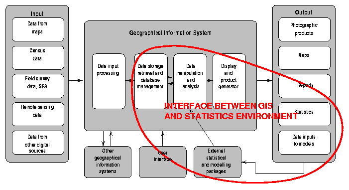
Figure 1. Major components of a geographical information system and their relationships with each other.
The components of geographical information systems involved in integration with data analysis and statistical programming environments are shown in Fig. 1. It is of course possible to reduce or extend the kinds of GIS activity that could benefit from integration with statistics, from screening input data for extreme outliers to mapping - for example interactive choice of class intervals for thematic maps of continuous or count data.
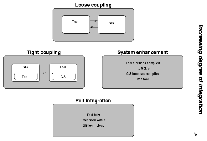
Figure 2. Integration of tools in a geographical information system.
From initially interfacing R and GRASS through loose coupling, transferring data through ad hoc text files, the work presented here involves tight coupling, running R from within the GRASS shell environment, and additionally system enhancement, by dynamically loading compiled GIS library functions into the R executable environment.
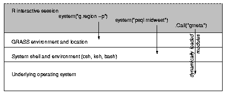
Figure 3. Layering of shell, GRASS and R environments.
Because R has developed as an interactive language with clear scoping rules and sophisticated handling of environment issues, while GRASS is a collection of partly coordinated separate programs built on common library functions, constructing working interfaces with GRASS has been challenging. One of the advantages of working with open source projects in this context has been that occasionally poorly documented functions can be read as source code, and when necessary thoroughly instrumented and debugged, to establish how they actually work. This is of particular help when interface functions are being written, since the mindsets and attitudes of several different communities of programmers need to be established.
The key insight needed to establish the interface is that GRASS treats the shell environment as its basis, assigning values to shell variables on initiation which are used by successive GRASS programs, all of which are started with the values assigned to these variables. These name the current location and mapset, and these in turn point to session and default metadata on the location's regional extent and raster resolution, stored in a fixed form in the GRASS database - a collection of directories under the current location. Since GRASS simply sets up a shell environment, initiating specified shell variables, all regular programs, including R, can in principle be run from within GRASS, in addition to GRASS programs themselves. Finally, R has a system(command), where command is a string giving the command to be invoked, and this command is executed in the shell environment in which R itself was started. This means that system() can be used from within R to run GRASS (and other) programs, including programs requiring user interaction. Alternatively, the tcltkgrass GUI front-end can be started before (or from) R, giving full access to GRASS as well as R. This is illustrated in Fig. 3.
Furthest to the right in Fig. 3 is the use of GRASS library functions called from R through dynamically loaded shared libraries. The advantage of this is to speed up interaction and to allow R to be enhanced with GRASS functionality, in particular reading GRASS data directly into R objects. Dynamically loaded shared libraries also increase the speed of operations not vectorised within R itself, especially for loops. Vectors are the basic building blocks of R (note: 1-based vectors!), so many operations are inherently fast, because data is held in memory. However, reading the R interpreted and compiled code (for the base library), as well as the documentation on writing extension packages gives a good idea of where compiling shared libraries may be worth the extra effort involved.
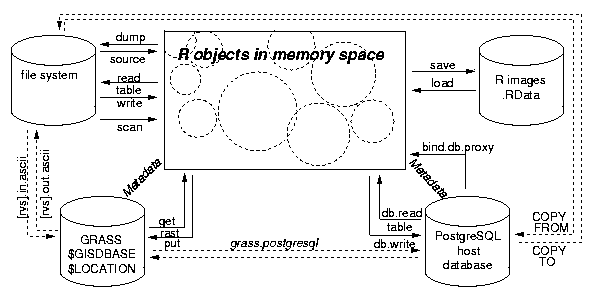
Figure 4. Feasible routes for data transfer between R, GRASS and PostgreSQL.
Native R supports the input and output of ascii text data, especially in the most frequently used form of data frame objects. These have a tabular form, with rows corresponding to observations, each with a character string row name, and columns to variables, each again with a string column name. Data frames contain numeric vectors and factors (which may be ordered), and can also contain character vectors; factors are an R object class of some importance, and are integer-valued, with 1-base integers pointing to the string label vector attribute. The read.table() function is however a memory hog, since reading in large tables with character variables for conversion to factors can use up much more memory than is necessary. The scan() function is more flexible, but data frames are certainly among the most used objects in R. Data frames differ from matrices in that matrices only contain one data type.
R objects may be output for re-entry with the dump() function, and entered using source(), both for functions and data objects. The R memory image may also be saved to disk for loading when a work session resumes, or for transfer to a different workstation. Every user of R has been caught by problems provoked by inadvertently loading an old image file, .RData in the working directory on start-up, in particular an apparent lack of memory despite little fresh data being read in.
There are a number of variants of data entry into R, and work is progressing on interfacing S family languages to RDBS (James, 2000), within the Omega project. Other read.table() flavours are also available, for example for *.csv files. In the following sub-sections, we will describe how the R/GRASS interface has been developed.
As an example, we can examine the code of the sites.get() function. The main part of the function is:
FILE <- tempfile("GRtoR")
system(paste("s.out.ascii -d sites=", slist, " > ", FILE, sep=""))
data <- read.table(FILE, na.strings="*")
unlink(FILE)
where slist is a valid GRASS sites database file. The logic of this snippet is simple: create a temporary file name; write the GRASS sites data to that file using s.out.ascii, read the file into an R data frame using read.table(), and finally remove the temporary file. It is worth noting that GRASS site file formats have been changing, and are not yet fully stabilised. It seems that site, line and polygon geometry has adequate support in GRASS, but that associating attribute values, especially multiple attribute values, with spatial objects is not yet stable. Maybe this is because of the raster nature of the system, in which the relationships between spatial objects and attribute values are handled very thoroughly.
The first step in using the interface is to initialise the grassmeta metadata structure, which contains information about the extent and raster resolution of the current region; in interpreted mode, this is taken from g.region. As can be seen below, two raster layers, elevation in metres and land use (for a small part of the Spearfish region), have been selected for transfer to R, but differ in resolution. The interface - like GRASS programs in general - assumes that the user needs the current resolution, not the initial resolution of the map layer. While the GRASS database holds 26600 cells for landuse and 294978 for elevation.dem, the transferred data follows the current region, with 106400 cells. Resampling is carried out by the underlying GRASS database functions for reading raster rows. Also note that landuse has been made into an R ordered factor. For comparison with the compiled interface, system times for the functions are reported for a lightly loaded 90MHz Pentium running RedHat Linux 6.2.
> library(GRASS)
Running in /usr/local/grass-5.0b/data/spearfish/rsb
> system("g.region -p")
projection: 1 (UTM)
zone: 13
north: 4928000
south: 4914000
west: 590000
east: 609000
nsres: 50
ewres: 50
rows: 280
cols: 380
> system.time(G <- gmeta(interp=TRUE))
[1] 0.03 0.00 0.69 0.21 0.10
> summary(G)
Data from GRASS 5.0 LOCATION spearfish with 380 columns and 280
rows;
UTM, zone: 13
The west-east range is: 590000, 609000, and the south-north: 4914000,
4928000;
West-east cell sizes are 50 units, and south-north 50 units.
> system("r.info landuse")
+----------------------------------------------------------------------------+
| Layer: landuse
Date: Mon Apr 13 10:13:08 1987 : |
| Mapset: PERMANENT
Login of Creator: grass
|
| Location: spearfish
|
| DataBase: /usr/local/grass-5.0b/data
|
| Title: Land Use ( Land Use )
|
|----------------------------------------------------------------------------|
|
|
| Type of Map: cell
Number of Categories: 8
|
| Rows:
140
|
| Columns: 190
|
| Total Cells: 26600
|
| Projection: UTM
(zone 13)
|
|
N: 4928000 S: 4914000
Res: 100
|
|
E: 609000 W:
590000 Res: 100
|
|
|
| Data Source:
|
| Cell file produced by EROS Data Center
|
|
|
|
|
| Data Description:
|
| Shows land use for the area using the
Level II
|
|
|
| Comments:
|
| classification scheme devised by the
USGS.
|
|
|
+----------------------------------------------------------------------------+
> system("r.info elevation.dem")
+----------------------------------------------------------------------------+
| Layer: elevation.dem
Date: Tue Mar 14 07:15:44 1989 |
| Mapset: PERMANENT
Login of Creator: grass
|
| Location: spearfish
|
| DataBase: /usr/local/grass-5.0b/data
|
| Title: DEM (7.5 minute) ( elevation )
|
|----------------------------------------------------------------------------|
|
|
| Type of Map: cell
Number of Categories: 1840
|
| Rows:
466
|
| Columns: 633
|
| Total Cells: 294978
|
| Projection: UTM
(zone 13)
|
|
N: 4928000 S: 4914020
Res: 30
|
|
E: 609000 W:
590010 Res: 30
|
|
|
| Data Source:
|
| 7.5 minute Digital Elevation Model (DEM)
produced by the USGS
|
|
|
|
|
| Data Description:
|
| Elevation above mean sea level in meters
for spearfish database
|
|
|
| Comments:
|
| DEM was distributed on 1/2 inch tape
and was extracted using
|
| GRASS DEM tape reading utilities.
Data was originally in feet
|
| and was converted to meters using the
GRASS map calculator
|
| (Gmapcalc). Data was originally
supplied for both the
|
| Spearfish and Deadwood North USGS 1:24000
scale map series
|
| quadrangles and was patched together
using GRASS
|
|
|
|
|
+----------------------------------------------------------------------------+
> system.time(spear <- rast.get(G, rlist=c("elevation.dem", "landuse"),
+ catlabels=c(FALSE, TRUE), interp=TRUE))
[1] 13.50 0.20 47.05 7.32 0.51
> str(spear)
List of 2
$ elevation.dem: num [1:106400] NA NA NA NA NA NA NA NA NA
NA ...
$ landuse.f : Factor w/ 8 levels "residential",..:
NA NA NA NA NA NA NA NA NA NA ...
The current interface is for raster and site GIS data; work on an interface for vector data is proceeding, but is complicated by substantial infelicities in GRASS methods for joining attribute values of vector objects to position data. Changes in GRASS programs like v.in.shape and its relatives are occurring rapidly, and are also associated with the use of PostgreSQL for storing tables of attribute data. We will return to this topic in concluding.
> system.time(G <- gmeta(interp=FALSE))
[1] 0.01 0.00 0.10 0.04 0.01
> system.time(spear <- rast.get(G, rlist=c("elevation.dem",
"landuse"),
+ catlabels=c(FALSE, TRUE), interp=FALSE))
[1] 1.07 0.06 2.08 0.00 0.00
> str(spear)
List of 2
$ elevation.dem: num [1:106400] NA NA NA NA NA NA NA NA NA
NA ...
$ landuse.f : Factor w/ 9 levels "no data","resid..",..:
NA NA NA NA NA NA NA NA NA NA ...
A by-product of programming the raster interface in C has been the possibility of moving R factor levels across the interface as category labels loaded directly into the GRASS raster database structure. While incurring the cost of extra disk usage as compared to GRASS reclassing technology, raster file compression reduces the importance of this issue. In the case below of reclassifying the elevation data from Spearfish by quartiles, the Tukey five number summary, the resulting data file is actually smaller than its null file, recording NAs.
> elev.f <- as.ordered(cut(spear$elevation.dem,
+ breaks=fivenum(spear$elevation.dem), include.lowest=TRUE))
> str(elev.f)
Factor w/ 4 levels "(1.07e+03,1..",..: NA NA NA NA NA NA NA NA
NA NA ...
> class(elev.f)
[1] "ordered" "factor"
> col <- rainbow(4)
> plot(G, codes(elev.f), reverse=reverse(G), col=col)
> legend(c(590000,595000), c(4914000, 491700),
+ legend=levels(elev.f)[1:2], fill=col[1:2], bty="n")
> legend(c(597000,602000), c(4914000, 491700),
+ legend=levels(elev.f)[3:4], fill=col[3:4], bty="n")
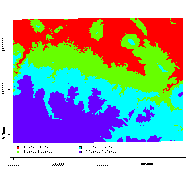
Figure 5. plot.grassmeta() object dispatch function used to display classified elevation map in R.
> rast.put(G, "elev.f", elev.f, "Tranfer of fivenum elevation classification",
+ cat=TRUE)
> system("ls -l $LOCATION/cell/elev.f")
-rw-r--r-- 1 rsb
users 9909 Jul 15 14:09 elev.f
> system("r.info elev.f")
+----------------------------------------------------------------------------+
| Layer: elev.f
Date: Sat Jul 15 14:09:14 2000 |
| Mapset: rsb
Login of Creator: rsb
|
| Location: spearfish
|
| DataBase: /usr/local/grass-5.0b/data
|
| Title: Tranfer of fivenum elevation classification
( elev.f )
|
|----------------------------------------------------------------------------|
|
|
| Type of Map: raster
Number of Categories: 4
|
| Rows:
280
|
| Columns: 380
|
| Total Cells: 106400
|
| Projection: UTM
(zone 13)
|
|
N: 4928000 S: 4914000
Res: 50
|
|
E: 609000 W:
590000 Res: 50
|
|
|
| Data Source:
|
|
|
|
|
|
|
| Data Description:
|
| generated by rastput()
|
|
|
|
|
+----------------------------------------------------------------------------+
> table(elev.f)
elev.f
(1.07e+03,1.2e+03] (1.2e+03,1.32e+03] (1.32e+03,1.49e+03]
(1.49e+03,1.84e+03]
26517
26162
26354
26301
> system("r.report elev.f units=c")
r.stats: 100%
+-----------------------------------------------------------------------------+
|
RASTER MAP CATEGORY REPORT
|
|LOCATION: spearfish
Sat Jul 15 14:10:54 2000|
|-----------------------------------------------------------------------------|
| north:
4928000 east: 609000
|
|REGION south: 4914000 west:
590000
|
| res:
50 res: 50
|
|-----------------------------------------------------------------------------|
|MASK:none
|
|-----------------------------------------------------------------------------|
|MAP: Tranfer of fivenum elevation classification (elev.f in rsb)
|
|-----------------------------------------------------------------------------|
|
Category Information
| cell|
|#|description
| count|
|-----------------------------------------------------------------------------|
|1|(1.07e+03,1.2e+03] . . . . . . . . . . . . . . . . . . . . .
. . . .| 26517|
|2|(1.2e+03,1.32e+03] . . . . . . . . . . . . . . . . . . . . .
. . . .| 26162|
|3|(1.32e+03,1.49e+03]. . . . . . . . . . . . . . . . . . . . .
. . . .| 26354|
|4|(1.49e+03,1.84e+03]. . . . . . . . . . . . . . . . . . . . .
. . . .| 26301|
|*|no data. . . . . . . . . . . . . . . . . . . . . . . . . . .
. . . .| 1066|
|-----------------------------------------------------------------------------|
|TOTAL
|106400|
+-----------------------------------------------------------------------------+
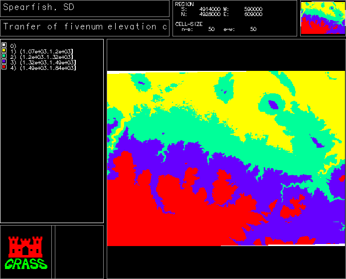
Figure 6. GRASS display of R reclassed elevation.
One specific problem encountered in writing the interface is a result of mixing two differing system models: R requires that compiled code uses its error handling routines returning control to the interactive command line on error, while not only the GRASS programs but also their underlying libraries quite often simply exit() on error. This of course also terminates R, if the offending code is dynamically loaded, behaviour that is hazardous for R data held in objects in memory. Patches have been applied to key functions in the GRASS libgis.a library, and are both available from the CVS repository and will be in the released source code from 5.0 beta 8.
The RPgSQL is loaded after starting R:
> library(RPgSQL)
In our case we are starting R within GRASS to access GRASS data directly.
Before using the RPgSQL, an empty database needs to be created. This can
be done externally:
$ createdb test
or within R:
> system("createdb geodata")
The user must have permission to create databases. This can be specified
when creating a PostgreSQL user. (createuser command).
Then the connection to the database "geodata" has to be established:
> db.connect("localhost", "5432", "geodata")
Within this database "geodata" a set of tables can be stored. The database may of course be initiated externally, by copying data into previously created tables using the standard database tools, for example psql. The key goal of this form of data transfer is to use the GRASS-PostgreSQL interface to establish the database prior to work in R, and to use the R-PostgreSQL interface to pass back results for further work in GRASS.
An issue of some weight - and as yet not fully resolved in the GRASS-PostgreSQL
interface - is stewardship of the GIS metadata: GRASS assumes that it "knows"
the metadata universe, but this is in fact not "attached" to data stored
in the external database. It is probable that fuller use of this solution
to data transfer will require the choice of one of two future routes: the
registration of a GRASS metadata table in PostgreSQL (somewhat similar
to the use of gmeta() above); or the implementation of a GRASS
daemon serving metadata, and possibly data in general, to programs requesting
it. Although these are serious matters, and indicate that this is far from
resolved, attempts to interface through a shared external database do illuminate
the problems involved in a very helpful way.
> data("soildata")
In case the user has the data frame available loaded into R, it can
be moved further to PostgreSQL. It is recommended to use the "names" parameter
to avoid name convention conflicts with PostgreSQL:
> db.write.table("soildata", name="soildata", no.clobber=F)
Now the memory of R can be freed of the "soildata" data frame as it
was copied to PostgreSQL:
> rm(soildata)
To re-connect the data set to R, the proxy binding follows. Due to
the proxy method the data interchange between PostgreSQL and R is established:
> bind.db.proxy("soildata")
> summary("soildata")
Table name: soildata
Database: geodata
Host: localhost
Dimensions: 10 (columns) 1000 (rows)
The data access is different to the common data access as the proxy
methods only delivers selected data to the R system. An example for selective
data access is by addressing rows and columns:
> selected.data <- soildata[25:27,]
> selected.data
area perimeter g2.i stonr
horiz humus pH
25 5232.31 322.597 26
20 Ah 20 5.4
26 75256.80 1986.950 27 10
Ap1 10 5.6
27 5276.81 285.431 28
6 aAp 6 4.8
or by addressing fields through column names:
> humus.data <- soildata[["humus"]]
> humus.data
[1] 1.45 1.33 1.45 2.71 1.45 1.33 1.33 1.45 1.74 1.45 2.81
1.33 1.78 1.69 2.51
[16] 1.33 1.77 1.33 2.41 0.00 0.00 1.62 1.33 2.10 2.10 1.69 2.38
1.33 2.51 1.33
[31] 1.34 2.10 0.00 1.92 0.00 1.45 1.33 2.10 0.00 1.33 2.51 2.71
1.69 1.33 2.71
[46] 2.10 1.33 1.69 2.10 2.71 1.34 2.71 2.71 2.10 1.33 1.33 2.68
1.74 1.33 1.45
[61] 2.71 2.38 2.68 1.69 1.33 1.33 1.33 1.33 1.33 2.71 2.71 2.10
2.71 2.10 1.69
[76] 1.33 1.45 1.33
These selected data (or results from calculations) can be written as
a new table to the PostgreSQL database, too:
> db.write.table(selected.data, name="selected_data", no.clobber=F)
To read it back the command:
> bind.db.proxy("selected_data")
will be used.
Although users do not need to know SQL query language, it is possible
to send SQL statements to the PostgreSQL backend:
> db.execute("select * from humus", clear=F)
> db.read.column("humus", as.is=T)
Calculations are performed by addressing the rows to use in calculation.
To calculate the mean of
> mean(na.omit(soildata$humus[1:1000,]))
[1] 1.723718
Finally the data cleanup can be done. The command
> rm(soildata)
would remove the data frame from R memory, and
> db.rm("soildata", ask=F)
removes the table from the PostgreSQL database "geodata". The
> db.disconnect()
disconnects the data link between R and the PostgreSQL backend.
The new R-PostgreSQL interface offers rather unlimited data capacities to overcome the memory limitations within R. A basic problem of the current implementation is the large speed decrease caused by the proxy method. The recently introduced ODBC driver has not so far been tested to compare it to the RPgSQL route. Perhaps future versions of the PostgreSQL-driver will offer fast data exchange as it is required for GIS analysis.
It is important to know is that the GRASS data can be stored directly into the DBMS and, using the proxy binding, connected to R. The GRASS modules v.to.db and r.to.db will be published with next GRASS 5 beta8 release.
CORBA interposes a broker between interfaced software systems, so that the interface can be abstracted from a many-to-many situation to a many-to-CORBA-to-many model, also known as a three-tier model. A .Corba() function has been experimentally written for S-like languages, as a way of handling interfacing with ORDBMS, and to ease access to data on distributed platforms. The same .Corba() interface has been refered to by Duncan Temple Lang on the r-help discussion list as a convenient route to farming out R compute tasks across multiple executing R instances. IDL is a facility for standardising the ways applications declare their willingness and abilities to interact with others - a comparable technology is DCOM in the Windows world.
Using markup languages for data transfer has a long history, and is still developing. Perhaps one major reason for looking at XML in the GIS context is the OGC RFC11 Geography Markup Language (GML) 1.0, published in December 1999 in connection with work on web mapping. This differentiates between geometry collections, feature collections, and spatial reference systems at the DTD (Document Type Definition) level. The underlying logic is that an XML object should contain all of its metadata - that it is self-describing, or pointers to DTD links providing access to metadata, so that applications exchanging XML streams or files can rely on knowing what the arriving or departing data are. XML is one of the active areas in the Omega project, and both DTD's and XML files based on them can be read into S-like languages, and data can be written to an XML file using the specified DTD. As with the CORBA work in the Omega project, this is still experimental, but it is clear that there are many shared themes of interest with the GIS and GeoComputing community.
The following example demonstrated how to calculate a trend surface
of the distributed pH value within the Spearfish region. The above mentioned
PostgreSQL-support in R (RPgSQL) is used again to overcome the memory limitations
within R.
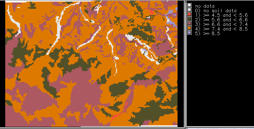
Figure 7: Soil pH-values within the Spearfish region.
For starting up the systems, R is called within GRASS software:
grass5.0beta
R --vsize=30M --nsize=500K
Then the GRASS/R interface is loaded:
> library(GRASS)
> G <- gmeta()
To generate the trend map of pH-values, the pH-map will be read into
R environment:
> soilsph <- rast.get(G, "soils.ph", c(F))
> names(soilsph) <- c("ph")
> gc()
          free   total (Mb)
Ncells  367838  512000  9.8
Vcells 3218943 3932160 30.0
Depending on the resolution previously set in GRASS, the demand on memory is different. The next step is to copy the map "soilsph" into the PostgreSQL database system. A new database needs to be created to store the new pH-value table:
It is recommended to use the "names" parameter in db.write.table to
avoid name conflicts (as PostgreSQL rejects special character within table
names).
To simulate a later access to the stored table, we disconnect from
the SQL-backend and reconnect again without loading the dataset. Using
the "gc()" command we can watch the memory consumption of our dataset.
> db.disconnect()
> rm(soilsph)
> gc()
free total
(Mb)
Ncells 364378 512000 9.8
Vcells 3884663 3932160 30.0
The memory in R is rather free now. We connect back to PostgreSQL and
now, instead of reading in the table, a proxy binding is set as described
above:
> db.connect("localhost", "5432", "soils_ph_db")
> bind.db.proxy("soilsph")
> gc()
free total
(Mb)
Ncells 364395 512000 9.8
Vcells 3882569 3932160 30.0
There is nearly no change in memory requirement. A small problem is
the decrease in speed as the requested data have to pass the proxy system.
> summary(soilsph)
Table name: soilsph
Database: soils_ph_db
Host: localhost
Dimensions: 1 (columns) 26600 (rows)
Selected data can be accessed by specifying the minimum and maximum
row numbers:
> soilsph[495:500]
I.data.
495 4
496 4
497 4
498 4
499 4
500 3
But usually we would want to analyse the full dataset (here equal to
our soils map with distributed pH-value). To find out the maximum number
of values alias raster cells, we can enter:
> maxrows <- dim(soilsph)[1]
This "maxrows" value we need to address the rows for further calculations.
To generate the trend surface of pH-values within the project area a data
frame containing x-, y-coordinates and the z-value (here: pH) has to be
set, and zero values set to NA:
> soils.ph.frame <- data.frame(east(G), north(G), soilsph[1:maxrows])
> soilsph$ph[soilsph$ph == 0] <- NA
> names(soils.ph.frame) <- c("x", "y", "z")
> summary(soils.ph.frame)
x
y
z
Min. :590100 Min. :4914000
Min. : 1.000
1st Qu.:594800 1st Qu.:4918000 1st
Qu.: 3.000
Median :599500 Median :4921000 Median
: 4.000
Mean :599500 Mean :4921000
Mean : 3.379
3rd Qu.:604300 3rd Qu.:4924000 3rd
Qu.: 4.000
Max. :609000 Max. :4928000
Max. : 5.000
NA's :977.000
To calculate the cubic trend surface, we have to mask NULL values from
calculation. The functions to fit the trend surface through the data points
is provided by "spatial" package:
> library(spatial)
> ph.ctrend <- surf.ls(3, na.omit(soils.ph.frame))
The map values of the trend surface are stored in object "ph.trsurf".
Finally the resulting trend surface can be visualized by either using contour
lines or selecting a solid surface.
> plot(G, trmat.G(ph.ctrend, G, east=east(G), north=north(G)),
+ reverse=reverse(G), col=terrain.colors(20))
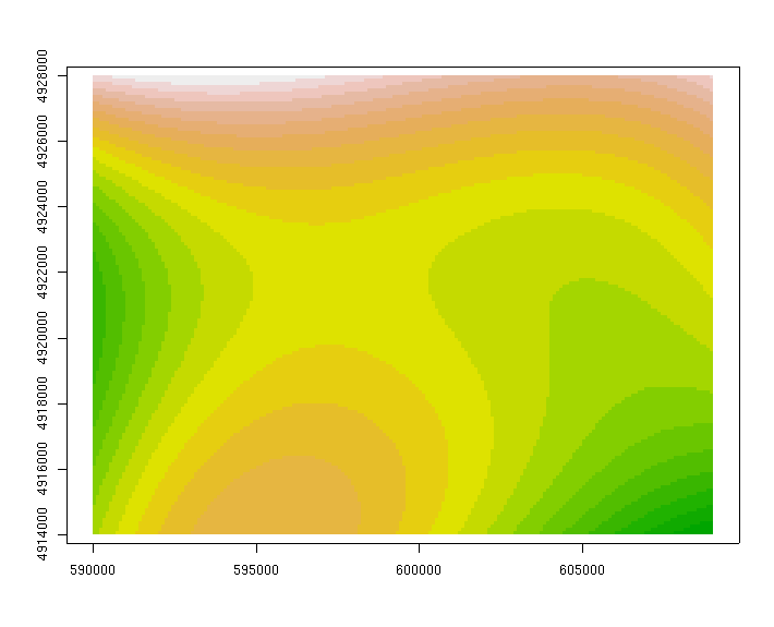
Figure 8: Trend surface of pH-value within Spearfish region.
> system("r.average base=landcov cover=topo output=avheight")
r.stats: 100%
percent complete: 100%
> system("r.report landcov units=c,h")
r.stats: 100%
+-----------------------------------------------------------------------------+
|
RASTER MAP CATEGORY REPORT
|
|LOCATION: leics
Mon Jul 17 15:07:39 2000|
|-----------------------------------------------------------------------------|
| north:
322000 east: 456000
|
|REGION south: 310000 west:
444000
|
| res:
50 res: 50
|
|-----------------------------------------------------------------------------|
|MASK:none
|
|-----------------------------------------------------------------------------|
|MAP: Land Cover / Land Use (landcov in PERMANENT)
|
|-----------------------------------------------------------------------------|
|
Category Information
| cell| |
|#|description
|count| hectares|
|-----------------------------------------------------------------------------|
|1|Industry . . . . . . . . . . . . . . . . . . . . . . . . .|
1671| 417.750|
|2|Residential. . . . . . . . . . . . . . . . . . . . . . . .|
6632| 1658.000|
|3|Quarry . . . . . . . . . . . . . . . . . . . . . . . . . .|
555| 138.750|
|4|Woodland . . . . . . . . . . . . . . . . . . . . . . . . .|
1749| 437.250|
|5|Arable . . . . . . . . . . . . . . . . . . . . . . . . . .|22913|
5728.250|
|6|Pasture. . . . . . . . . . . . . . . . . . . . . . . . . .|16816|
4204.000|
|7|Scrub. . . . . . . . . . . . . . . . . . . . . . . . . . .|
6558| 1639.500|
|8|Water. . . . . . . . . . . . . . . . . . . . . . . . . . .|
706| 176.500|
|-----------------------------------------------------------------------------|
|TOTAL
|57600|14,400.000|
+-----------------------------------------------------------------------------+
> system("r.report avheight units=c,h)
r.stats: 100%
+-----------------------------------------------------------------------------+
|
RASTER MAP CATEGORY REPORT
|
|LOCATION: leics
Mon Jul 17 15:09:45 2000|
|-----------------------------------------------------------------------------|
| north:
322000 east: 456000
|
|REGION south: 310000 west:
444000
|
| res:
50 res: 50
|
|-----------------------------------------------------------------------------|
|MASK:none
|
|-----------------------------------------------------------------------------|
|MAP: (untitled) (avheight in rsb)
|
|-----------------------------------------------------------------------------|
|
Category Information
| cell| |
|
#|description
|count| hectares|
|-----------------------------------------------------------------------------|
| 76.300667-76.582816|from to . . . . . . . . . . .
. . . .| 6632| 1658.000|
| 83.354396-83.636545|from to . . . . . . . . . . .
. . . .| 1671| 417.750|
| 99.154749-99.436898|from to . . . . . . . . . . .
. . . .| 706| 176.500|
|103.669135-103.951285|from to . . . . . . . . . . . . .
. .|22913| 5728.250|
|133.012648-133.294797|from to . . . . . . . . . . . . .
. .|16816| 4204.000|
|134.987692-135.269842|from to . . . . . . . . . . . . .
. .| 555| 138.750|
| 142.60572-142.887869|from to . . . . . . . . . . . . .
. .| 1749| 437.250|
|147.966554-148.248703|from to . . . . . . . . . . . . .
. .| 6558| 1639.500|
|-----------------------------------------------------------------------------|
|TOTAL
|57600|14,400.000|
+-----------------------------------------------------------------------------+
Using the interface, we move the two layers to R, landcov as a factor, and topo as a numeric vector. The tapply() function lets us apply the declared function mean() to the subsets of the first argument grouped by the second, giving the results we need. The counts of cells by land use type are given by table(), which we can next covert to hectares using the metadata on cell resolution. Finally, we construct a boxplot of elevation by land use, making box width proportional to the numbers of cells in each land use class (note that the first, empty, count is dropped by subsetting c2[2:9]).
> library(GRASS)
Running in /usr/local/grass-5.0b/data/leics/rsb
> G <- gmeta()
> leics <- rast.get(G, c("landcov", "topo"), c(T, F))
> str(leics)
List of 2
$ landcov.f: Factor w/ 9 levels "Background","In..",..: 6
6 6 6 6 6 6 6 6 6 ...
$ topo : num [1:57600] 80 80 80 80
80 80 80 80 78 76 ...
> c1 <- tapply(leics$topo, leics$landcov.f, mean)
> c2 <- table(leics$landcov.f) * ((G$ewres*G$nsres) / 10000)
> colnames(c3) <- c("Average Height", "Total Area")
> c3[2:9,]
Average Height Total Area
Industry
83.61101 417.75
Residential 76.30066
1658.00
Quarry
135.25405 138.75
Woodland 142.94454
437.25
Arable
104.02143 5728.25
Pasture 133.48335
4204.00
Scrub
148.24870 1639.50
Water
99.26912 176.50
> boxplot(leics$topo ~ leics$landcov.f, width=c2[2:9], col="gray")
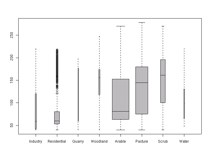
Figure 9. Boxplot of elevation in metres by land cover classes, NW Leicestershire; box widths proportional to share of land cover types in study region.
It is of course difficult to carry out effective data analysis, especially graphical data analysis, in a GIS like GRASS, but boxplots such as these are of great help in showing more of what the empirical distributions of cell values look like.
Over and above substantive analysis of map layers, we are often interested in checking the data themselves, particularly when they are the result of interpolation of some kind. Here we use a plot of the empirical cumulative distribution function to see whether the contours used for digitising the original data are visible as steps in the distribution - as Figure 10 shows, they are.
> library(stepfun)
> plot(ecdf(leics$topo), verticals=T, do.points=F)
> for (i in seq(40,240,20)) lines(c(i,i),c(0,1),lty=2, col="sienna2")
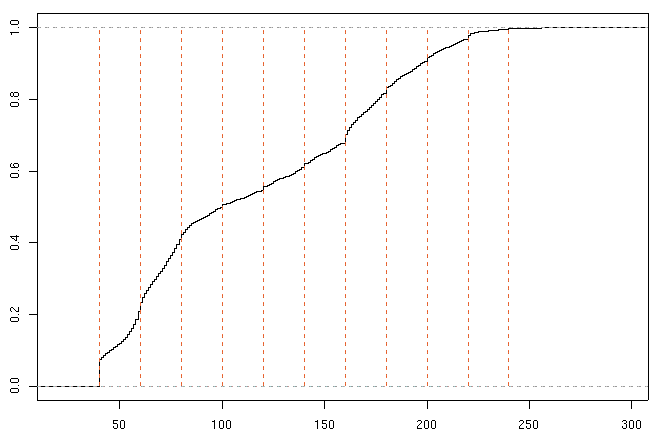
Figure 10. Empirical cumulative density function of elevation values in metres, NW Leicestershire; also known as hypsometric integral.
A further tool to apply in search of the impact of interpolation artifacts is the density plot over elevation. A conclusion that can be drawn from Figure 11 is that only at above a bandwidth of over 6 metres do the artifacts cease to be intrusive.
> plot(density(leics$topo, bw=2), col="black")
> lines(density(leics$topo, bw=4), col="green")
> lines(density(leics$topo, bw=6), col="brown")
> lines(density(leics$topo, bw=8), col="blue")
> for (i in seq(40,240,20)) lines(c(i,i),c(0,0.015),lty=2, col="sienna2")
> legend(locator(), legend=c("bw=2", "bw=4", "bw=6", "bw=8"),
+ col=c("black", "green", "brown", "blue"), lty=1)
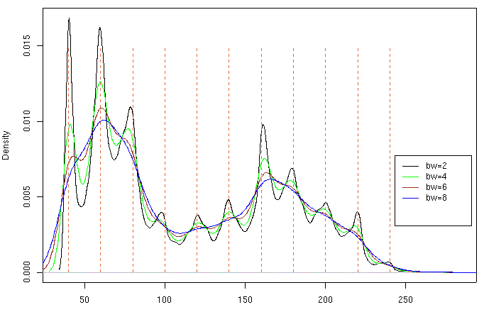
Figure 11. Density plots of elevation in metres from bandwidth 2 to 8 metres showing the effects of interpolating from digitised contours.
The data set used for the exampled given here was included in the materials of the ESDA with LISA conference held in Leicester in 1996. The data are for the five midwest states of Illinois, Indiana, Michigan, Ohio, and Wisconsin, and stems from the 1990 census. The boundary data stems from the same source, but the units used are not well documented; there are 437 counties included in the data set. For this presentation, the position data were transformed from an unknown projection back to geographical coordinates, and projected from these to UTM zone 16. R regression and prediction functions were used to carry out a second order polynomial transformation, as in GRASS i.rectify2 used for image data. Projection was carried out using the GMTmapproject program.
It did not prove difficult to import the reformatted midwest.arc file into GRASS with v.in.arc, but joining it to the midwest.pat data file was substantially more difficult. As an alternative, the midwest.arc was converted using awk to a line segment input file for map.builder - a collection of simple awk and shell scripts and two small programs compiled from C: intersect and gdbuild. This, after the removal of duplicate line segments identified by intersect, permitted the production of a polylines file and a polygon file. These were converted in awk to a form permitting R lists to be built using split(). From there, getting R to do maps was uncomplicated, by reading in the files, and using splitting them. The split() function is an R workhorse, being central to tapply() used above, and is an optimised part of R's internal compiled code. It splits its first argument by the second, returning a list with elements containing vectors with the component parts of the first argument. A short utility function was used - mkpoly() - to build a new list of closed polygons from the input data.
> mwpl <- scan("map.builder/mw.polylines", list(id=integer(0),
+ x=double(0), y=double(0)))
> mwpe <- scan("map.builder/mw.polygon", list(pid=integer(0),
+ edge=integer(0)))
> s.mwpe <- split(mwpe$edge, as.factor(mwpe$pid))
> sx.mwpl <- split(mwpl$x, as.factor(mwpl$id))
> sy.mwpl <- split(mwpl$y, as.factor(mwpl$id))
> polys <- vector("list", length(s.mwpe))
> for (i in 1:length(s.mwpe))
+ polys[[i]] <- mkpoly(sx.mwpl, sy.mwpl, s.mwpe,
i)
The label point data from the midwest.arc file were extracted using awk and read into an R list. Another utility function - polynames() - was used to employ the inout() function from the Splancs library to find which label points belong to which polygons.
> mwcpl <- scan("map.builder/mw.lab", list(lab=integer(0),
+ x=double(0), y=double(0)))
> library(splancs)
> pnames <- polynames(mwcpl, polys)
The result of running polynames() is then used to join the polygon list to the attribute data for the vector to be mapped, through thw which() function, another R workhorse, fast even though interpreted, and also used in polynames(). The data for mapping has to be quantized, here using the quantile() function, but a vector of user-defined break-points could as well have been used. If the quantized data is not assigned class ordered, the user may find that level labels are not assigned in intuitive order, potentially making legends difficult to construct.
> mwdata <- read.table("midwest.tab", T, row.names=2, sep=",")
> ophp <- as.ordered(cut(mwdata$php, breaks=quantile(mwdata$php,
+ seq(0,1,0.1)), include.lowest=TRUE))
> id.ophp <- data.frame(mwdata$id, ophp)
> pointers <- integer(nrow(mwdata))
> for (i in 1:length(pointers))
+ pointers[i] <- which(pnames$lab == id.ophp$mwdata.id[i])
> gr <- gray(18:9/20)
> library(MASS)
> eqscplot(c(100000, 1100000), c(100000, 1300000), type="n")
> for (i in 1:nrow(id.ophp)) + polygon(polys[[pointers[i]]],
col=gr[codes(id.ophp$ophp[i])])
> legend(c(-107000, 119300), c(476000, 95000),
+ legend=levels(id.ophp$ophp), fill=gr)
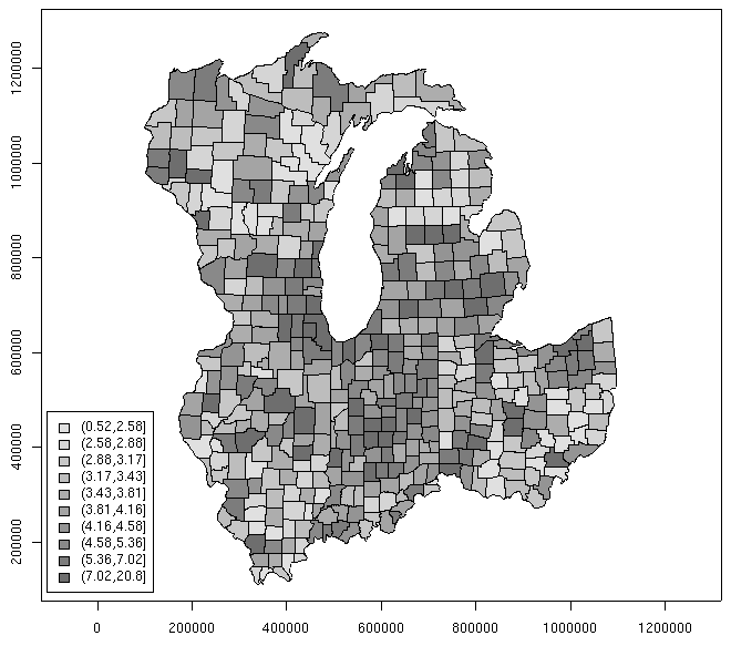
Figure 12. Percentage of persons aged 25 years and over with professional or higher degrees, 1990, five Mid-West states.
A further example is to use the pointer vector to paint polygons meeting chosen attribute conditions - this is analogous to the examples given in the GRASS-PostgreSQL documentation. The R which() function is not unlike the SQL SELECT command, but returns the row numbers of the objects found in the data table, rather than the requested tuples. To retrieve selected columns, their names or indices can be given in the columns field of the [<rows>, <columns>] access operator for data frames. As may have been noticed, there is also an [[<list elements>]] access operator for lists, so that polys[[pointers[i]]] returns the pointers[i]'th list element of polys, which is itself a list of two numeric vectors of equal length, containing the x and y coordinates of the polygon. When we attempt to label the five counties with percentages of persons 25 years and over with professional and higher degrees over 14 percent, we have to go back through the chain of pointers to find the label point coordinates originally used to label the polygons at which to plot the text.
> where <- which(mwdata$php > 14)
> str(where)
int [1:5] 10 39 155 181 275
> mwdata[where, c("pop", "pcd", "php")]
pop pcd php
CHAMPAIGN (IL) 173025 41.29581 17.75745
JACKSON (IL) 61067 36.64367 14.08989
MONROE (IN) 108978 37.74230 17.20123
TIPPECANOE (IN) 130598 36.24544 15.25713
WASHTENAW (MI) 282937 48.07851 20.79132
> pointers <- integer(nrow(mwdata))
> for (i in 1:length(pointers))
+ pointers[i] <- which(pnames$lab == mwdata$id[i])
> eqscplot(c(100000, 1100000), c(100000, 1300000), type="n")
> for (i in 1:nrow(mwdata)) polygon(polys[[i]])
> for (i in which(mwdata$php > 4.447 & mwdata$php <= 10))
+ polygon(polys[[pointers[i]]], col="yellow")
> for (i in which(mwdata$php > 10 & mwdata$php <= 14))
+ polygon(polys[[pointers[i]]], col="orange")
> for (i in which(mwdata$php > 14))
+ polygon(polys[[pointers[i]]], col="red")
> texts <- rownames(mwdata)[where]
> text(mwcpl$x[pnames$id[pointers[where]]],
+ mwcpl$y[pnames$id[pointers[where]]], texts, pos=4, cex=0.8)
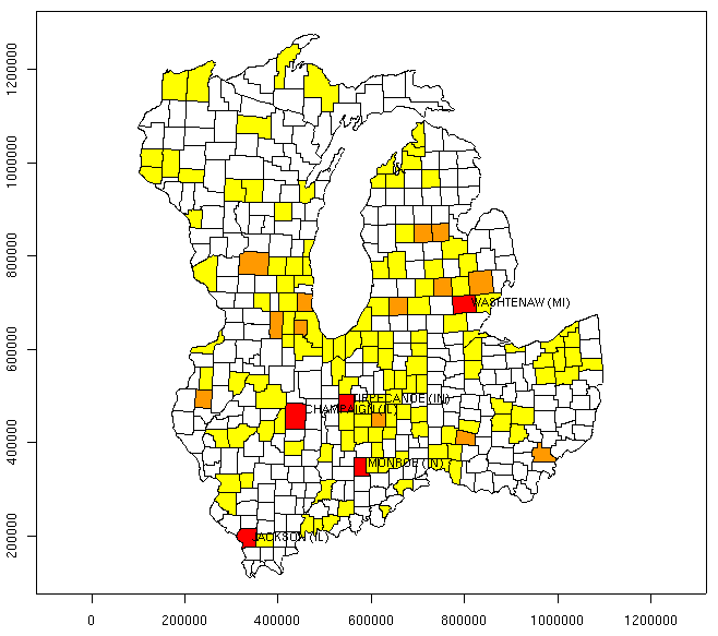
Figure 13. Finding counties with high percentages of persons aged 25 years and over with professional or higher degrees, 1990, five Mid-West states.
To conclude this subsection, the maps package county database is used to map the same variable; the database is plotted using unprojected geographical coordinates at present. The problem that arises is that the map() function fills the polygons with specified shades or colours in the order of the polygons in the chosen database, and that joining the data table attribute rows to the polygon database is thus a point of weakness. Here we see that the county database returns a vector of 436 names of counties in the five states, while the EsdaLisa Mid-West data reports 437. After translating the county names into the same format, the %in% operator is used to locate the county name or names not in the county database. Fortunately, only one county is not matched, Menominee(WI), an Indian Reservation in the North East of the state. The next task is to use its label coordinates from the Mid-West data set to find out in which county database polygon it has been included. While there must be a way of reformatting the polygon data extracted from map(), use was made here of awk externally, and then split() and inout() as above. The county from the county database in which Menominee has been subsumed is its neighbour Shawano, with which it is aggregated on the relevant variables before mapping. In fact, both Menominee and Shawano were both in the bottom decile before aggregation, with Menominee holding the lowest rank for percentage aged 25 and over holding higher or professional degrees, and Shawano ranked 33. The aggregated Shawano comes in at rank 20 of the 436 county database counties.
> library(maps)
> mw <- read.table("midwest.tab", T, sep=",", row.names=2)
> cnames <- map("county", c("illinois","indiana","michigan",
+ "ohio","wisconsin"), namesonly=T)
> str(cnames)
chr [1:436] "illinois,adams" "illinois,alexander" "illinois,bond"
...
> mwnames <- tolower(rownames(mw))
> str(mwnames)
chr [1:437] "adams (il)" "alexander (il)" "bond (il)" "boone (il)"
...
> ntab <- c("(il)", "(in)", "(mi)", "(oh)", "(wi)")
> names(ntab) <- c("illinois", "indiana", "michigan", "ohio",
"wisconsin")
> ntab
illinois indiana michigan
ohio wisconsin
"(il)" "(in)"
"(mi)" "(oh)" "(wi)"
> for (i in 1:length(mwnames)) {
+ x <- unlist(strsplit(mwnames[i], " "))
+ nx <- length(x)
+ mwnames2[i] <- paste(names(which(ntab ==
x[nx])), ",", x[1], sep="")
+ if (nx > 2) for (j in 2:(nx-1)) mwnames2[i]
<- paste(mwnames2[i],
+ x[j], sep=" ")
+ }
> str(mwnames2)
chr [1:437] "illinois,adams" "illinois,alexander" "illinois,bond"
...
> inn <- logical(length(mwnames2))
> for (i in 1:length(mwnames2)) inn[i] <- mwnames2[i] %in% cnames
> which(!inn)
[1] 405
> mw[405,]
id area pop dens white black
ai as or pw pb
MENOMINEE (WI) 3020 0.021 3890 185.2381 416
0 3469 0 5 10.69409 0
pai pas por pop25
phs pcd
php poppov
MENOMINEE (WI) 89.17738 0 0.1285347 1922 62.69511
7.336108 0.5202914 3820
ppoppov ppov ppov17 ppov59
ppov60 met categ
MENOMINEE (WI) 98.20051 48.6911 64.30848 43.31246 18.21862
0 LHR
> mwpts <- read.table("~/proj/papers/gc00/esda1.dat", T, row.names=1)
> mwpts[which(mwpts$id == 3020),]
id x
y e
n
51 3020 13.983 10.2195 -88.6893 44.9859
> cpolys <- map("county", c("illinois","indiana","michigan","ohio",
+ "wisconsin"), namesonly=F, plot=F, fill=T)
> str(cpolys)
List of 3
$ x : num [1:7381] -91.5 -91.5 -91.5 -91.5
-91.4 ...
$ y : num [1:7381] 40.2 40.2 40.0 40.0
39.9 ...
$ range: num [1:4] -92.9 -80.5 37.0 47.5
> summary(cpolys$x)
Min. 1st Qu. Median Mean 3rd
Qu. Max. NA's
-92.92 -89.16 -87.15 -86.80 -84.47
-80.51 435.00
> write.table(cbind(cpolys$x, cpolys$y), "cpolys.dat", quote=F,
+ row.names=F, col.names=F)
> system(paste("awk \'BEGIN{i=1}{if ($1 != \"NA\") print i, $1,
$2;",
+ "else i++;}\' cpolys.dat > cpolys1.dat"))
> cpolys1 <- scan("cpolys1.dat", list(id=integer(0), x=double(0),
+ y=double(0)))
Read 6946 lines
> str(cpolys1)
List of 3
$ id: int [1:6946] 1 1 1 1 1 1 1 1 1 1 ...
$ x : num [1:6946] -91.5 -91.5 -91.5 -91.5 -91.4 ...
$ y : num [1:6946] 40.2 40.2 40.0 40.0 39.9 ...
> cp.x <- split(cpolys1$x, as.factor(cpolys1$id))
> cp.y <- split(cpolys1$y, as.factor(cpolys1$id))
> cpolys2 <- vector(mode="list", length=length(cp.x))
> for (i in 1:length(cp.x)) { cpolys2[[i]] <- list(x=unlist(cp.x[i]),
+ y=unlist(cp.y[i]))
+ attr(cpolys2[[i]]$x, "names") <- NULL
+ attr(cpolys2[[i]]$y, "names") <- NULL
}
> res <- logical(length=length(cpolys2))
> for (i in 1:length(cpolys2)) res[i] <-
+ inout(as.points(x=-88.6893, y=44.9859), as.points(cpolys2[[i]]))
> which(res)
[1] 423
> cnames[423]
[1] "wisconsin,shawano"
> mw[toupper("shawano (wi)"),]
id area pop dens white black
ai as or pw
SHAWANO (WI) 3039 0.054 37157 688.0926 35251
42 1762 70 32 94.87041
pb pai
pas por pop25
phs pcd
SHAWANO (WI) 0.1130339 4.742041 0.1883898 0.08612105 24271 69.45326
14.80780
php poppov ppoppov ppov ppov17
ppov59 ppov60 met
SHAWANO (WI) 2.455605 36389 97.9331 11.29737 14.93227 9.105113
11.94953 0
categ
SHAWANO (WI) AAR
> which(rownames(mw) == toupper("shawano (wi)"))
[1] 424
> p25 <- mw$pop25
> php <- mw$php
> ahp <- (p25*php)/100
> p25.436[1:404] <- p25[1:404]
> p25.436[405:422] <- p25[406:423]
> p25.436[424:436] <- p25[425:437]
> p25.436[423] <- sum(p25[c(405,424)])
> ahp.436[1:404] <- ahp[1:404]
> ahp.436[405:422] <- ahp[406:423]
> ahp.436[424:436] <- ahp[425:437]
> ahp.436[423] <- sum(ahp[c(405,424)])
> php.436 <- (100*ahp.436)/p25.436
> br <- quantile(mw$php, seq(0,1,0.1))
> ophp.436 <- as.ordered(cut(php.436, breaks=br, include.lowest=TRUE))
> gr <- gray(18:9/20)
> map("county", c("illinois","indiana","michigan","ohio","wisconsin"),
+ fill=T, col=gr[codes(ophp.436)])
> legend(c(-94.4, -91.6), c(36.94, 40.0),
+ legend=levels(ophp), fill=gr, bty="n", cex=0.8)
> map("county", "wisconsin,shawano", color="red", add=T)
> mw$php[c(405,424)]
[1] 0.5202914 2.4556055
> codes(ophp[c(405,424)])
[1] 1 1
> rank(mw$php)[c(405,424)]
[1] 1 33
> php.436[423]
[1] 2.313595
> codes(ophp.436[423])
[1] 1
> rank(php.436)[423]
[1] 20
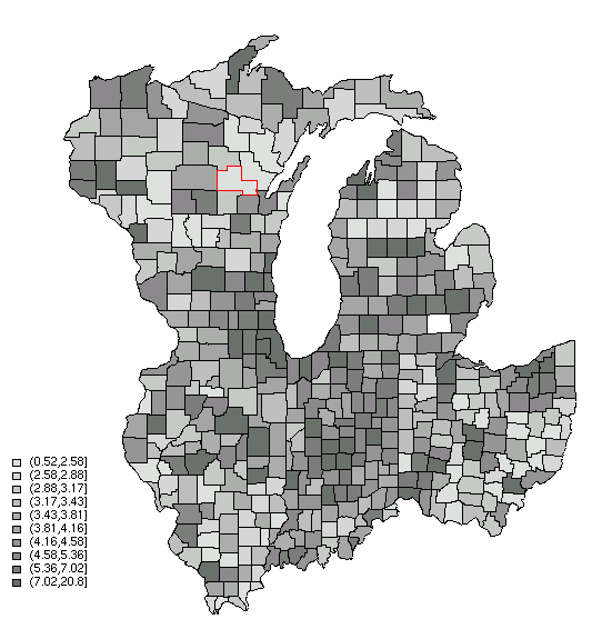
Figure 14. Percentage of persons aged 25 years and over with professional or higher degrees, 1990, five Mid-West states, mapped using the R maps package.
This worked example points up the difficulty of ignoring absent metadata needed for integrating data tables with mapped representations, and suggests that further work on the maps package is needed to protect users from assuming that they are mapping what they assume. It is very possible that the RPgSQL link could be used to monitor the joining of map polygon databases to attribute database tables.
While progress is being made in GRASS on associating site, line and area objects with attribute values, not least in the context of the GRASS-PostgreSQL link, it is still far from easy to join geographical objects to tables of attributes using object id-numbers. Migration to the new sites format in GRASS is not fully complete, and even within this format, it is not always clear how the attribute table should be used. Similar reservation hold for vector map layers.
In the past, attempts have been made to use PostgreSQL's geometric data types, which support the same kind of object model as the OGC Simple Feature model used in GML. They are not in themselves built topologies, but to move from cleaned elements to topology is feasible. GRASS has interactive tools for accomplishing this, but on many occasions GRASS users import vector data from other sources, support for which is increasing, now also with support for storing attribute tables in PostgreSQL. In the example above, use was made of tools from the S map.builder collection to prepare cleaned and built topologies for the Midwest data set. Here again, it was necessary to combine both automation of topology construction with object labelling to establish a correct mapping from clean polygons to attribute data, as also in GRASS v.in.arc and other import programs.
These concerns are certainly among those that increase the relevance of work in the Omega project on interfacing database, analysis and presentation systems, including three-tier interfaces using CORBA/IDL. They also indicate a possible need for rethinking the GRASS database model, so that more components can be entrusted to an abstract access layer, rather than to hard-wired directory trees - work that is already being done for attribute data.
On the data analysis side, most of the key questions have been taken up and are being investigated in the Omega project, especially those of importance for raster GIS interfaces like very large data sets. R's memory model is most effective for realistically sized statistical problems, but is restricting for applications like remote sensing or medical imaging, when special solutions are needed (particularly to avoid using data frames). This issue of scalability, and ways of parallelising R tasks for distribution to multiple compute servers deserves urgent attention, and - combined with the R-PostgreSQL link to feed compute nodes with subsets of proxied data tables - is not far off.
Finally, we would like to encourage those who feel a need or interest in open source development to contribute - it is rewarding, and although combining projects with closed deliverables with apparent altruism may seem difficult, experience of the open source movement indicates that, on balance, projects advance better when difficulties are shared with others, who may have met simmilar difficulties before.
Becker, R. A. 1993. Maps in S. Bell Labs, Lucent Technologies, Murray Hill, NJ.
Becker, R. A. and Wilks, A. R. 1995. Constructing a geographical database. Bell Labs, Lucent Technologies, Murray Hill, NJ.
Bivand, R. S., 1999. Integrating GRASS 5.0 and R: GIS and modern statistics for data analysis. In: Proceedings 7th Scandinavian Research Conference on Geographical Information Science, Aalborg, Denmark, pp. 111-127.
Bivand, R. S. 2000. Using the R statistical data analysis language on GRASS 5.0 GIS database files. Computers & Geosciences, 26, pp. 1043-1052.
Bivand, R. S. and Gebhardt, A. (forthcoming) Implementing functions for spatial statistical analysis using the R language. Journal of Geographical Systems.
Chambers, J. M. 1998. Programming with data. (New York: Springer).
Ihaka R, 1998 R: past and future history. Unpublished paper.
Ihaka, R. and Gentleman, R. 1996 R: a language for data analysis and graphics. Journal of Computational and Graphical Statistics, 5, 299-314.
Jones, D. A. 2000 A common interface to relational databases from R and S - a proposal. Bell Labs, Lucent Technologies, Murray Hill, NJ (Omega project).
Neteler, M. 2000 Advances in open-source GIS. Proceedings 1st National Geoinformatics Conference of Thailand, Bangkok.
Venables, W. N. and Ripley, B. D. 1999 Modern applied statistics with S-PLUS. (New York: Springer); (book resources).