Return to GeoComputation 99 Index

Investigating the spatial variation of radon in soil geostatistically

M. A. Oliver1, and A. L. Kharyat2
1Department of Soil Science, The University of Reading, Whiteknights, Reading RG6 6DW, U.K.
2Department of Physics, College of Science, Taiz University, Republic of Yemen
E-mail: m.a.oliver@rdg.ac.uk

Abstract

Concern about possible links between emissions of radon and certain types of malignant disease has led to surveys to measure radon concentrations in the soil and in dwellings. There is little information about the spatial resolutions over which radon varies. Such information is needed to sample effectively to measure radon for spatial prediction. To explore the spatial variation of radon we measured its concentration in the soil gas using solid state nuclear track detection in a radon affected area in the English Midlands. Three surveys are described. The first was a nested survey with seven stages near to Buxton in Derbyshire in an area comprising two main lithological units and a minor one. The other surveys were just to the South of the former on one of these lithologies, the Monsal Dale limestone. One was an irregularly scattered sample in two dimensions where radon concentration, particle size distribution and elevation were recorded. The other was along a transect 2 km long. In addition to radon concentration, ground conductivity and slope angle were measured every 20 m. The results suggest that although geology exerts a strong control on the variation, other factors are involved. There appear to be relations between radon concentration in the soil and elevation, soil depth, and particle size distribution.

1. Introduction

Exposure to natural sources of radiation has become an important issue in terms of radiological protection. Much of this comes from 222Rn and its solid, short-lived daughter products, 218Po, 214Pb and 214Bi. The National Radiological Protection Board, NRPB, (1992) estimates that radon accounts for approximately 50 % of a person's annual dose of radiation from all sources in the United Kingdom. Radon is a ubiquitous naturally occurring radioactive gas that may be emitted from any rock that contains uranium or thorium. The radon potential for a given region is likely to be the result of a combination of properties of the underlying rocks and of the soil, such as the distribution of uranium and radium, porosity, permeability, and moisture content, as well as meteorological and seasonal variation.

Interest in the spatial distribution of radon is increasing because of putative links with malignant disease. Elevated levels of radon in houses are thought to lead to increased malignancy, in particular lung cancer (Clarke and Southwood, 1989; Green et al., 1992). Other epidemiological studies internationally have suggested that exposure to radon might be a cause of several forms of cancer including certain childhood cancers (Henshaw et al., 1990; Lucie, 1989). To substantiate these correlations and to relate radon values to estimates of the risk of malignancy (Oliver et al., 1992) information is required about the spatial variation in radon; however, Bowie and Bowie (1991) have commented on the lack of substantive data on the localized exhalation rates of Rn.

To describe the radon emanation in a given area reliably we need to determine what kind of estimates are feasible. It has already been accepted generally that radon emission is affected by geology, and this led Ball et al. (1991) to suggest that a few well-sited measurements could be used to predict its values over a larger area. Essentially such estimates of radon are the mean concentrations for a given spatial class related to the underlying geology. In some areas, however, there is likely to be considerable local variation in radon concentration within geological units because it depends on factors other than lithology, such as atmospheric pressure, temperature, soil moisture, CO2 concentration in the soil, porosity, and so on. In this case, estimates based on classification would result in too much loss of information, especially for comparing radon concentration with the incidence of disease.

If geology accounts for all of the spatially correlated variations, then it is sensible to use the within-stratum means as predictors. If not, then some method of local estimation such as kriging (Matheron, 1965; 1971) should be considered. The choice of the method of prediction for radon depends on knowing something about the structure of its spatial variation: both of these also have implications for sampling. Appropriate sampling is affected by the spatial resolution of the variation. The body of techniques embodied in geostatistics (Matheron, 1965; 1971) provide the tools to enable us to determine the structure of the spatial variation and to choose an appropriate method of local estimation to estimate radon values optimally, and to design optimal sampling schemes for kriging.

We measured soil radon concentration using solid state nuclear track detection (SSNTD) in two parts of Derbyshire in the English Midlands, near Buxton. We used a nested survey and analysis with seven stages to determine the structure of radon spatial variation on three lithologies. With this information we designed two further surveys on a single lithology: the first was an irregularly distributed sample in two dimensions and the other was a regular sample along a transect. In addition to radon concentration for the survey in two dimensions, soil particle size distribution and elevation were recorded, and the transect ground conductivity and slope angle were measured.

2. Radon in soil gas

Radon forms in rocks and soil that contain uranium or thorium. Rocks have generally been thought to be the major source, for example the granites of Devon and Cornwall (England) are important sources of radon. The amounts exhaled in those counties are among the largest in the United Kingdom (NRPB, 1992). Peake and Hess (1987) and Hung et al. (1994) also suggest that the soil itself is an important source. This is supported further by the findings of Jones (1995). He described the Rn source in soil as either dispersed, i.e., occurring as single atoms of U disseminated randomly throughout the soil mass, or as concentrated U in minerals such as zircon, sphene, and apatite. By examining the tracks on the detectors, Jones (1995) concluded that U disseminated throughout the soil is more likely to produce Rn than that trapped in the minerals. He also found that the radon concentration in the air in basements in Illinois was related to dispersed soil U, but not to total U.

The half life of radon is 3.82 days, which is another factor suggesting that the radon in houses is more likely to have formed in the soil than in the underlying rock. This is corroborated by Nero et al. (1990) who estimated that soil contributes more than 90% of Rn in houses, and by Akerblom et al. (1984) and Swedjemark (1986) who also reported that large concentrations of Rn in the soil gas were associated with large concentrations indoors; therefore, radon concentration is generally measured either in the soil or in homes. Radon moves into buildings because of a negative pressure differential, and because of a large concentration gradient between the building and bedrock or soil. Reimer (1991) says that the rate of migration of radon in soil can greatly influence indoor radon concentration. Ball et al. (1991) suggested that the concentration of radon in houses is likely to relate fairly closely to that in the soil although there is no well established method of estimating radon levels in individual dwellings based on soil radon data. Agard and Gundersen (1991) went further in suggesting that there are direct correlations between uranium, radium, radon in soil gas, and indoor radon concentrations. Reimer et al. (1991) also suggested that geology and soil gas radon are useful indicators of indoor radon concentration. These relations are unlikely to be straightforward, however, and there is much scope for investigating this further. We considered that soil radon might provide a reasonable guide for assessing the potential for large radon concentrations in homes. Radon, 222Rn and thoron, 220Rn, are usually produced in approximately equal quantities, but the latter is often ignored because its contribution to the overall dose of radiation is relatively small. For both the soil and buildings there are many other factors, in addition to the spatial variation in the source elements, that complicate the spatial variation of radon emanation. For example, the spatial variation in soil permeability, porosity, CO2 concentration in the soil gas, moisture content, and atmospheric pressure affect its emanation. Soil moisture content can increase radon emanation but, if the soil pores become saturated, emission is inhibited. Carbon dioxide acts as a carrier gas for radon in soil which can enhance its concentration in the soil atmosphere (Ball et al. , 1991). The values inside buildings depend on structural characteristics, ventilation rates, aerosol concentration, central heating, building materials, and the habits of the inhabitants.

To avoid the complications associated with buildings, we decided to measure concentrations of radon in the soil. We used the well-established `can-technique' - a simple passive detection system using solid-state nuclear track detectors. Cylindrical cans, each containing a 2 cm by 2 cm piece of CR-39 plastic detector, were placed in the ground at a depth of 50 cm and covered with a 70 cm length of PVC tubing (closed at the top end) at each sampling location. Full details of this technique are given by Durrani et al. (1991). The detectors were left in situ for approximately three works - long enough for the 222Rn (T1/2 = 3.82 d) to reach equilibrium with its long-lived parent, radium, and for a significant number of tracks resulting from its a-decay to be registered on the plastic. In each case the detectors were etched electrochemically (Durrani et al., 1991) under standard conditions to enlarge the tracks for counting with an optical microscope.

3. Estimating radon spatially

Spatial information is generally obtained at selected locations, sampling points. The sampling design and intensity of sites to measure radon concentration will depend on how radon varies spatially, and the method of estimation that we would either like to use, or that is appropriate. Since it seems likely that radon varies more or less continuously in geographical space, it can be regarded as a regionalized variable (Matheron, 1965; Badr et al. , 1993) and can be analysed geostatistically.

There are two basic approaches to estimating the values of properties at unsampled sites from fragmentary information: classification and interpolation. The one that we adopt might depend on the kind of estimates we require or on what is feasible given the nature of the spatial variation. Estimation by some form of interpolation provides more local detail about a property's spatial variation, but this approach is suitable only if the data are spatially dependent or correlated.

Classification is the classical approach; it gives an estimate of the mean concentration for each spatial class or stratum, and the estimated value at each location in the class is the mean. Any spatial correlation is assumed to be accounted for by the classes and any residual variation within them is regarded as wholly random. The model for classification is: (1) where zij is the value of property Z at any point I in class j, m is the general mean of Z, aj is the difference between m and the mean of class j, and eij is a random component with zero mean and variance, w2, i.e., the within class variance.

The estimate of zij is the mean of the observations in class j: (2) where nj is the number of observations in class j. The estimator, zij is the weighted average of the observations in the class, with weights equal to nj.

If the classification accounts for all of the spatially dependent variation then the class mean is the best estimate of the property and we cannot do better; however, if there is spatially dependent variation remaining within the classes, then local detail is lost. In this situation a method of interpolation, such as kriging, should be used to avoid the loss of information. Voltz and Webster (1990) showed that if marked boundaries delimit areas of more or less continuous variation, then a combination of classification and kriging provides the best estimates.

A model of spatial variation for geostatistical estimation is: (3) where Z(x) is the random variable at x, v is the local mean of Z in the neighbourhood of x, and e(x) is a random term with an expectation of zero, and a variance such that for any two places x and x + h separated by a lag h is given by: (4) where g is the semivariance between two places a distance and direction h apart. If mv is constant locally, then equation (4) is equivalent to: (5) which defines the variogram of Z.

The variogram provides an unbiased description of the scale and pattern of spatial variation, the spatial model needed for kriging, and a basis for designing optimal sampling schemes (McBratney et al. , 1981). To estimate the variogram precisely, however, we need to have some idea of the order of magnitude of the spatial variation because it can reveal little more than a single order of magnitude of spatial resolution. Clues to the approximate resolution of the variation often are elusive because spatial properties vary in a complex way, and they can vary on scales that differ by several orders of magnitude simultaneously, i.e., nested variation. An efficient means of exploring the spatial structure of the variation at the outset is by a nested sampling scheme and hierarchical analysis of variance (Oliver and Webster, 1987; Badr et al., 1993; Oliver and Badr, 1995). In addition the reconnaissance variogram and that of regionalized variable theory can be used to suggest which approach is suitable for estimation. We describe and illustrate these approaches with three case studies.

4. Case studies

4.1. Derbyshire: nested survey

This survey followed a nested survey near to Hereford in the English Midlands on a single geological formation, the Old Red Sandstone (Devonian), Oliver and Badr (1995). Although this survey covered a wide range of sampling distances, 10 m to 7.5 km, all of the variation appeared to occur over distances less than 10 m. The results suggested that there was no structure in the variation, and that the values were fluctuating about the mean. It seemed that lithology was exerting the major control on soil radon variation, and that the mean Rn value for that lithology was a suitable predictor. Furthermore, methods of interpolation including kriging could not be used for prediction with these data because there was no spatial dependence. Another survey with samples every 20 m along a transect near to Nottingham (Oliver and Badr, 1995), also in the English Midlands, suggested that lithology accounted for all of the spatially dependent variation. A conventional variogram was computed from the radon concentrations in this case and it showed some spatial structure initially; however, when the effect of the different lithologies was taken into account, the variogram of the residuals from the class means showed no evidence of structure. Again in this example estimates based on the within-stratum mean would be the best possible.

To determine whether the mean Rn value for a given geological formation was the best predictor in general, we chose an area to the southeast of Buxton with two main types of rock and a third one that was less dominant, Figure 1. This area also has been declared a `radon affected area' recently by the NRPB (1992) suggesting that the number of homes with radon levels greater than the British Government's recommended Action Level of 200 Bqm-3 exceeds 1 %.

The predominant lithologies in the surveyed area are both marine limestones of Carboniferous age, the Bee Low formation and the Monsal Dale limestone, Figure 1, (Aitkenhead et al. , 1985). The Bee Low limestone is characterized by its homogeneity and limited faulting, whereas the Monsal Dale limestone is much more variable, fossiliferous and more densely faulted. There was a small area of the Longnor sandstone in the southwest of the region, Figure 1. We deliberately avoided sampling an igneous outcrop in the central part of our area to avoid complicating the analysis and results unduly.

Figure 1. Map showing the location of the nine main centres of the nested survey to measure soil radon near Buxton (England), and the solid geology of the region.

4.1.1. Theory of Nested Sampling

Youden and Mehlich (1937) devised a means of determining the spatial scale of variation over several orders of magnitude simultaneously by adapting classical multistage sampling. For a spatial property, the stages in the hierarchy could be represented by different distances between sampling points. The underlying theory then is that a single observation embodies variation contributed by each of the distances, including an unresolved variance for the smallest spacing. The contributions of each stage or sampling distance to the total variance can be determined by a hierarchical analysis of variance. The components of variance for each spacing from this analysis reveal over what part of the spatial scale most of the variation occurs. The advantage of this method is that several orders of magnitude of spatial scale can be covered in a single analysis. Since the effects of distance are assumed to be random, the appropriate model of the analysis of variance is Model II of Marcuse (1949).

For a design with m stages, the model of variation is (6) where zijk . . . m is the value of the mth unit in . . . , in the kth class at stage 3, in the jth class at stage 2, and in the Ith class at stage 1. The general mean is m; Ai is the difference between m and the mean of class i at the first stage; Bij is the difference between the mean of the jth subclass in class i and the mean of class i; and so on. The final quantity eijk . . . m represents the deviation of the observed value from its class mean at the last stage of subdivision. The quantities Ai, Bij, Cij, . . ., eijk . . . m are assumed to be independent random variables associated with stages 1, 2, 3, . . ., m, respectively, having means of zero and variances s12, s22, s32, . . ., sm2. The latter are the components of variance for each stage. The individual component for a given stage measures the variation attributable to that stage, and together they sum to the total variance: (7) A further advantage of the nested approach became clear when Miesch (1975) showed that, if the components of variance are accumulated, starting with the smallest spacing, they were equivalent over the same range of distances to the semivariances of regionalized variable theory, equation (5). For m stages of subdivision and distances d1, d2, . . ., dm, where d1 is the shortest distance at the mth stage and dm the largest distance at the first stage, the equivalence is given by: (8) and so on.

In practice the components are only rough estimates of the true semivariances because there are too few degrees of freedom from which to estimate each component. Nevertheless, the set of values provides a first approximation to the variogram, and a rough description of the way a property varies with increasing separation in a given region. It can indicate the range of spatial scales over which most of the variation is occurring. It is an ideal reconnaissance tool for discovering the approximate spatial scale before designing a more detailed survey to estimate the experimental variogram precisely (Oliver and Webster, 1986; 1987) or to plan a routine survey for mapping.

4.1.2. Unbalanced nested sampling scheme in Derbyshire

The area surveyed was to the south east of Buxton in the county of Derbyshire: the northwestern corner of the grid was at SK 408373 (National Grid reference). Youden and Mehlich's (1937) original sampling design was fully balanced, which results in a doubling of the sample size for each stage. For a design with many stages, the number of samples soon becomes prohibitively large for a reconnaissance survey; therefore, we followed Oliver and Webster (1986) and Webster and Boag (1992) in using an unbalanced nested scheme to achieve greater spatial resolution without increasing sampling excessively. Full replication at each stage is unnecessary because the mean squares for the lower stages are estimated much more precisely than those for the higher stages; therefore, economy can be achieved by replicating at only a proportion of the sampling sites. Sacrificing the balance means that estimating the components is somewhat more complex. Gower (1962) and Gates and Shiue (1962) have provided computational procedures for calculating the coefficients for an unbalanced design (see Oliver and Webster, 1990 for more detail).

Our unbalanced nested sampling design had seven stages, and covered an area of 56.25 km2. There were nine main centres, 3.75 km apart, at the nodes of a square grid, aligned with the National Grid: three were on the Bee Low limestone, five on the Monsal Dale limestone, and one on the Longnor Sandstone, Figure 1. The twelve samples associated with each centre were on one of the main lithologies so that we could assess their effect on radon concentration. The sampling intervals were in a four- fold geometric progression encompassing these sampling intervals: 3 750 m, 950 m, 240 m, 60 m, 15 m, 4 m and 1 m. From the nine main centres, all of the other points in the scheme were then located on random orientations as follows. A second site was placed 950 m away to provide the second stage. From each of these 18 sites another point was located 240 m away (stage 3). At stage 4, a sample was placed 60 m away from just half of the stage 3 sites. This procedure of replicating just half of the sampling points was repeated for stages 5, 6 and 7 at distances of 15 m, 4 m and 1 m, respectively. Figure 2 shows a plan of the sampling points for one of the main centres. There were 108 sampling sites in total. With a balanced nested scheme for nine main centres and seven stages we should have had 576 sampling points, hence we reduced our sampling effort by more than 80 %.

Figure 2. Spatial configuration of the twelve sampling points for one of the nine centres of the nested survey, Buxton, Derbyshire (England).

4.1.3. Analysis and results

There were considerable differences between the individual radon concentration values for each centre, for example for Centre I the smallest value was 2.3 kBqm-3 and the largest was 40.0 kBqm-3. The overall minimum and maximum were 1.3 kBqm-3and 50.3 kBqm-3, respectively, which is a difference of almost two orders of magnitude (Table 1). There are clear differences between the mean radon concentration of each of the main centres on the Bee Low limestone and those on the Monsal Dale limestone, and also between their overall mean values: that for the Bee Low limestone is 10.1 kBqm-3, whereas for the Monsal Dale it is 22.88 kBqm-3. The centre on the Longnor sandstone had the smallest mean concentration of 5.4 kBqm-3; however, the values for this centre were similar to those of the centres on the Bee Low limestone. The overall average radon concentration for this survey was 17.36 kBqm-3 (Table 1) which is considerably greater than the National average of approximately 10 kBqm-3. This is probably due to karstification by circulating ground water that increases the permeability of the limestone (O'Connor et al. , 1992).

Table 1. Summary statistics for nested survey in Derbyshire, England

The histogram of the radon concentration for the Buxton survey was bimodal, which suggested that it was reasonable to treat the samples on the Longnor sandstone as part of the population on the Bee Low limestone. The radon values were analysed using a hierarchical analysis of variance (see Webster and Oliver, 1990), and we incorporated an extra stage to represent the two main lithologies. Table 2 gives the sampling intervals for each stage in the survey, the components of variance and the percentage variance explained. The components of variance were accumulated starting at the lowest stage, and plotted against distance on a logarithmic scale to give the reconnaissance variogram, the solid line in Figure 3. There is virtually no residual variance that suggests that samples separated by 1 m are very similar. From this it was reasonable to assume that little of the variance is attributable to measurement error. Spatial dependence is evident in the variation of soil radon concentration between 1 m and 4 m--this stage accounts for 20% of the variance. Almost 29% of the variance is accounted for by variation over distances of 60 m and 240 m, but just over 46% is accounted for by differences in lithology.

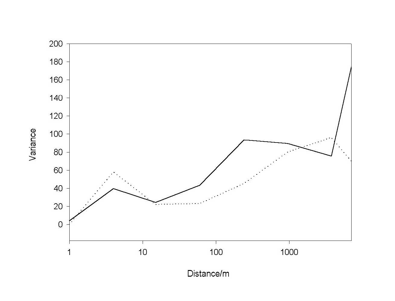
Figure 3. Accumulated components of variance plotted against distance on a logarithmic scale for soil radon concentration near Buxton, England: the solid line is for the raw data and the dotted one is for the residuals computed from the means of the lithologic units.

Table 2. Components of variance and percentage variance contributed by each stage from the nested survey of soil radon near to Buxton (Derbyshire, England).

This analysis shows that the underlying geology exerts a strong control on concentrations of radon in the soil gas; however, the reconnaissance variogram also suggests that there is spatial dependence within the lithological units. To determine whether this relates entirely to the underlying geology we also computed the components of variance for the residuals from the means of the two main lithologies. The reconnaissance variogram of the residuals is the dashed line in Figure 3: there is still strong spatial dependence over distances less than 4 m and between 60 m and 950 m. There is now no contribution to the variance by the stage representing the lithological units.

The nested survey suggests that although geology exerts a major control on the spatial variation of soil radon concentration, there is spatially dependent variation remaining within the lithological units. We explored this in more detail by sampling the Monsal Dale limestone only, and then by estimating radon concentration by kriging, as suggested by Voltz and Webster (1990).

4.2. Estimating radon concentration by kriging

We surveyed an area of 4 km2 just to the South of the area of the nested survey, near to Biggin (National Grid reference SK 41553594), and used the spatial information from the nested analysis to choose an appropriate sampling scheme. Ideally sampling on a grid is preferred for local estimation, but this was not feasible here because we had to take the landowners' convenience into account in locating the detectors as they had to be left in situ for at least 3 weeks. In addition we wanted some closely spaced samples so that we could compute the variogram as precisely as possible at the shorter separating distances. The sampling interval varied from 50 m to 250 m, which was well within the extent of spatial dependence indicated by the reconnaissance variogram. Figure 4 shows the locations of the 93 sampling points; they are fairly evenly spread over the area while ensuring that there would be enough comparisons at the shorter lags. The field and laboratory procedures were the same as before for determining the radon concentrations. In addition, the particle size distribution of a soil sample taken at a depth of 50 cm at each location was determined in the laboratory. The soil was sieved and the fine fraction, <2mm was dispersed in water containing Calgon. The proportions of sand, silt, and clay were then determined by settling (Klute, 1986). Elevation was recorded over the area at the same sites as were those at which radon was measured.

Figure 4. Map showing the locations of the sampling points for the survey in two dimensions near to Biggin, Derbyshire (England).

4.2.1. Variogram analysis and results

The summary statistics of the properties for the above survey are given in Table 3. Radon concentration was marginally skewed and we computed the experimental variogram from the raw data and the logarithmically transformed values conventionally using the usual computing formula: (9) where M(h) is the number of comparisons made at lag h. Since the data were irregularly distributed in two dimensions, the lag interval was determined by grouping the lag by both distance and direction so that there was a range in each that was applied to a nominal lag at the centre of the range (Webster and Oliver, 1990).

The variograms from the raw and transformed values were similar, and we chose to work with the raw data. Figure 5 shows the experimental semivariances as discrete points. A mathematical model was fitted to these values by weighted least squares approximation using MLP (Ross, 1987): a power function provided the best fit and this is shown as the solid line in Figure 5. The model parameters are given in Table 4. The equation for the isotropic power function is: (10) where w is the slope of the line, h is the lag, a is the exponent, and c0 is the nugget variance. The latter represents the spatially uncorrelated variation at the scale of the

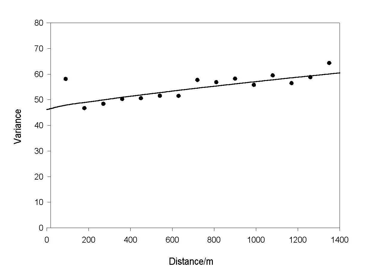
Figure 5. Variogram of radon concentration for Biggin, Derbyshire: the symbols are the experimental semivariances and the solid line is the fitted model.

Table 3. Summary statistics for the survey on a single lithology in two dimensions in Derbyshire

investigation. It encompasses spatially dependent variation over distances less than the shortest lag, measurement error, and any purely random variation. The nugget variance for this survey accounts for about 70 % of the total variance encountered, which shows that there is a large locally erratic component in the variation. The monotonically increasing section of the variogram represents the continuous component of the variation. The variogram is unbounded as we might expect for a single lithology.

Variograms were computed for elevation and the particle size fractions. That for elevation showed evidence of trend, which we removed by a linear function of the coordinates. We computed the variogram from the residuals and fitted an exponential model to this: its parameters are given in Table 4, and its equation is: (15) where c is the spatially dependent component and d is the distance parameter. The exponential model reaches its sill asymptotically; therefore, there is no absolute range or limit of spatial dependence. A working range, a, can be obtained as 3d, which is just over 1 km. Figure 6 show the experimental variogram with the fitted model.

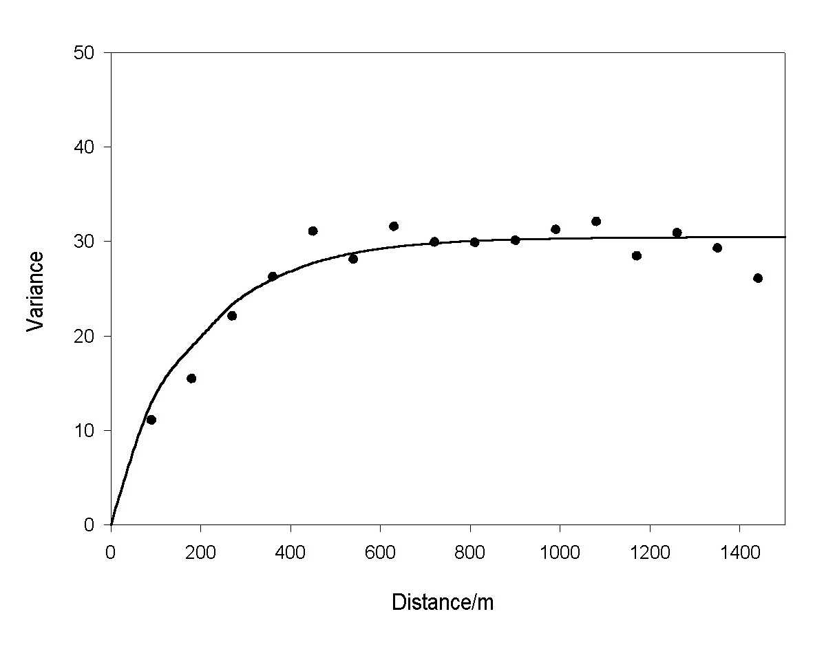
Figure 6. Variogram of the residuals from the trend for elevation (Biggin, Derbyshire): the symbols are the experimental semivariances and the solid line is the fitted model.

The variograms for the particle size fractions are erratic, possibly because there are too few samples. The variogram for sand could not be modelled satisfactorily, but those for clay and silt, Figures 7 and 8, respectively, were modelled with power functions as for the radon concentrations. Table 4 gives the parameters of these models.

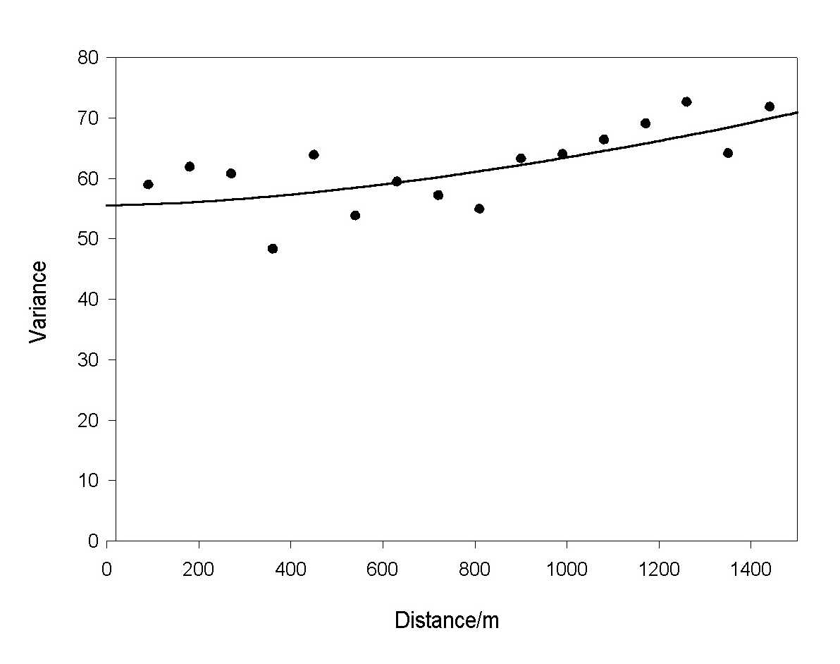
Figure 7. Variogram of percentage clay for Biggin, Derbyshire: the symbols are the experimental semivariances and the solid line is the fitted model.

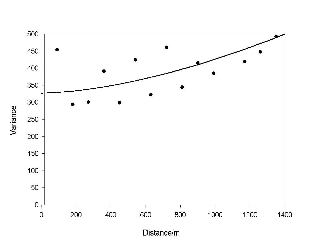
Figure 8. Variogram of percentage silt for Biggin, Derbyshire: the symbols are the experimental semivariances and the solid line is the fitted model.

Table 4. Variogram model parameters for properties measured in the two dimensional survey in Derbyshire.

4.2.2. Kriging

Kriging is essentially a method of weighted moving averages of the observed values of a property in a given neighbourhood, N. For a regionalized variable, Z, with measured values z(xI) at points (xi), i =1,2, . . . n, the equation for ordinary kriging is (11) where z(B) is the value estimated for a block B, and l are the weights assigned to the sampling points in the search neighbourhood, N, usually 16 to 25. Values can be estimated for points or blocks. In this case we estimated values on a fine square grid with a spacing of 50 m and over blocks of 100 m.

The kriging weights sum to 1 to ensure that the estimates are unbiased. The method is optimal in the sense that the weights are chosen to minimize the estimation or kriging variances, given by (12) where g(xi,xj) is the semivariance of Z between the Ith and the jth sampling points, (xi,B) is the average semivariance between the block and the ith sampling point, and g (B.B), is the average variance within the block, i.e., the within-block variance. Subject to the weights summing to one the estimation variance s2(B) is least when (13) The Lagrange multiplier, y, is introduced to achieve minimization. Equations (13) are the kriging equations that are solved to determine the weights that are then substituted in Equation (11) for estimating z(B). They also enable us to estimate the kriging variance by (14)

The estimation variances can be mapped in the same way as the estimated values and they provide an estimate of the reliability of the estimates.

4.2.3. Results of kriging

The block kriged estimates of radon concentration were contoured to produce the map in Figure 9a, and Figure 9b is map of the standard errors. The latter reflect the distribution of the samples, which are largest near to the edges of the region. Figure 9a shows that there is fairly continuous change in the values over the area as we should expect with an unbounded variogram. It is what we might expect on a single lithology. The radon concentrations decrease from West to East: they are largest in the low-lying area of the West and smallest on the plateau and spur in the East. The pattern of the variation is particularly distinctive because the radon concentrations appear to have an inverse relation with the relief. Figure 10 is a map of the elevation in the study area produced by kriging the residuals from the trend, followed by adding the linear trend function to the kriged estimates. The map shows a general decrease in the height of the land from East to West. There is a spur in the central part of the map and this is flanked by two small dry valleys. This relation between elevation and radon concentration is striking and it was unexpected.

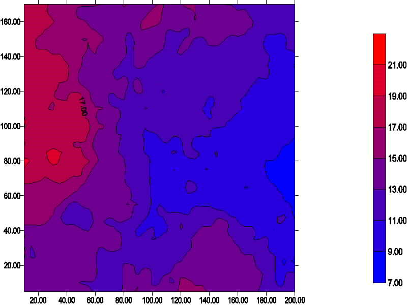Figure 9a

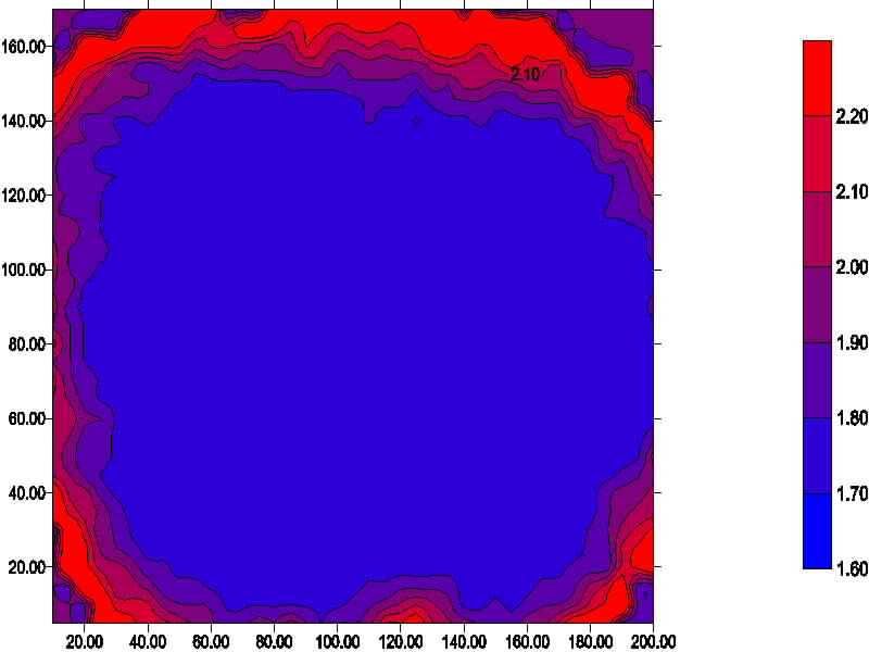Figure 9b

Figure 9. a) Map of kriged estimates of radon concentration near to Biggin, Derbyshire (England), and b) map of the standard errors for kriging.

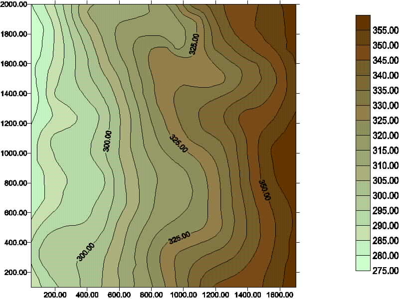
Figure 10. Map of kriged estimates of elevation after first removing the trend, kriging the residuals and adding the trend back to them, near to Biggin, Derbyshire (England).

Figures 11 and 12 show the contour maps of the kriged estimates of clay and silt contents for the area. There also appears to be a relation between clay content, radon concentration, and elevation: clay content is least in West and North West and greatest on the plateau and spur in the East. Silt also is least in the West and North West and greatest at the foot of the slope from the plateau and along the dry valleys. It seems that the large particle size fraction is associated with the large radon concentration in the soil. This relation needs to be examined further.

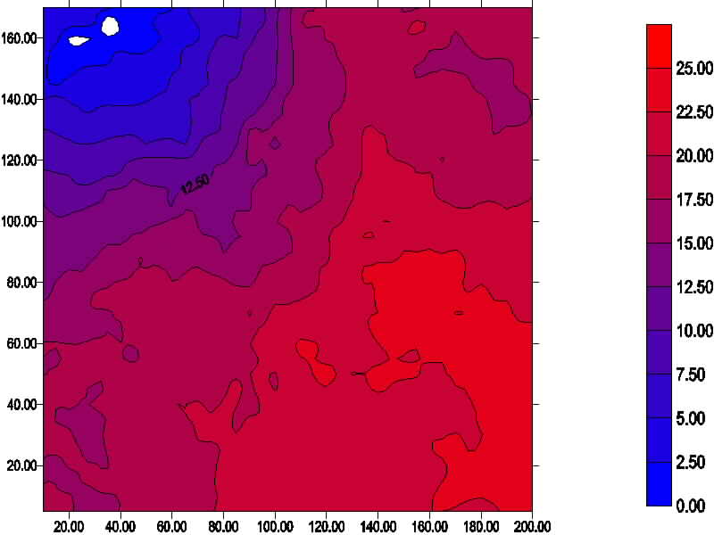
Figure 11. Map of kriged estimates of percentage clay near to Biggin, Derbyshire (England).

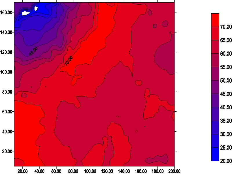
Figure 12. Map of kriged estimates of percentage silt near to Biggin, Derbyshire (England).

4.3. The transect survey

The map of the radon concentration, Figure 9, shows that there are factors other than the underlying geology that account for its spatial variation since this survey is on a single lithology. One possibility is that it is related to the depth of the soil or superficial materials to bedrock. This would support Jones' (1995) hypothesis that radon emanation is a function of the finely disseminated Uranium in the soil; therefore, one might contend that the thicker the soil the more U present and the greater the radon emanation.

To explore any possible relation between radon concentration and the depth of soil and superficial materials to the limestone bedrock, a transect survey was undertaken. It extended for 2 km from E-W from grid reference SK 160587. Radon was measured as before, but at an interval of 20 m. In addition, the slope angle was measured between the mid-sample positions on either side of the sampling point, and soil depth was measured electromagnetically.

4.3.1. Ground conductivity measurement

Electromagnetic techniques can be used for geological mapping and groundwater surveys (McNeill, 1980). There are two types: continuous wave and transient. Both methods produce a time varying magnetic field that induces eddy currents in any conducting body in the ground, which, in turn, produces a secondary magnetic field. We applied the continuous wave technique that measures the resultant of the primary and secondary fields using a continuous time varying magnetic field. The ratio of the secondary field, Hs to the primary field, Hp, is linearly proportional to the terrain conductivity that is determined directly by a conductivity meter. The apparent conductivity, sa: (15) where v = 2pf, and f is the frequency (Hz), mo is the permeability of the free space, and s is the intercoil spacing (m).

The ground conductivity was measured at 20 m intervals by a continuous electromagnetic wave using the Geonics EM31 equipment.

4.3.2. Results

The radon concentrations were plotted against sample spacing (Figure 13). They are very irregular, but it is possible to identify a weak trend from West to East with the values decreasing somewhat. Table 5 gives the summary statistics for radon and since they are skewed they were transformed to logarithms before computing the variogram. The experimental variogram, shown by the symbols in Figure14, has a sinusoidal from. We fitted a combined periodic with power function using MLP (Ross, 1987). The parameters of the best fitting model are given in Table 6, and its equation is: (16) in which the parameters a and b determine the amplitude and the phase of the wave, andl is its wavelength.

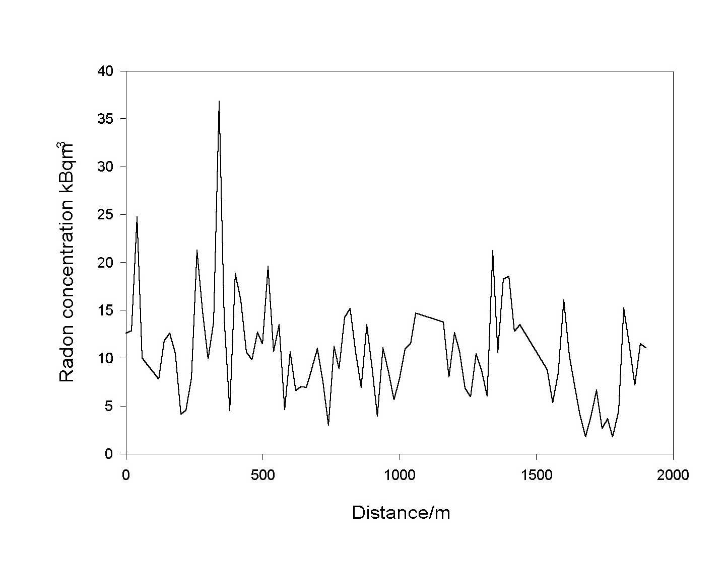
Figure 13. Graph of radon concentrations plotted against sampling position along the transect near to Biggin, Derbyshire (England).

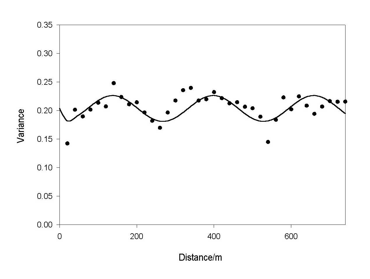
Figure 14. Variogram of radon concentration for the transect near to Biggin, Derbyshire: the symbols are the experimental semivariances and the solid line is the fitted model.

The ground conductivity measurements were plotted against sampling position (Figure 15). There is a weak trend from West to East with conductivity values decreasing. This seems to suggest that the soil is deeper in the West then in the East. The spikes in the conductivity values along the transect can be explained in several ways: the soil and superficial materials are not homogeneous and their conductivity can vary; the presence of highly conductive man-made objects, such as pipes, which seem unlikely in fields, or they reflect the karst topography of the limestone with deep overwidened joints being filled with soil, etc., and have a larger conductivity. The latter is the favoured explanation.

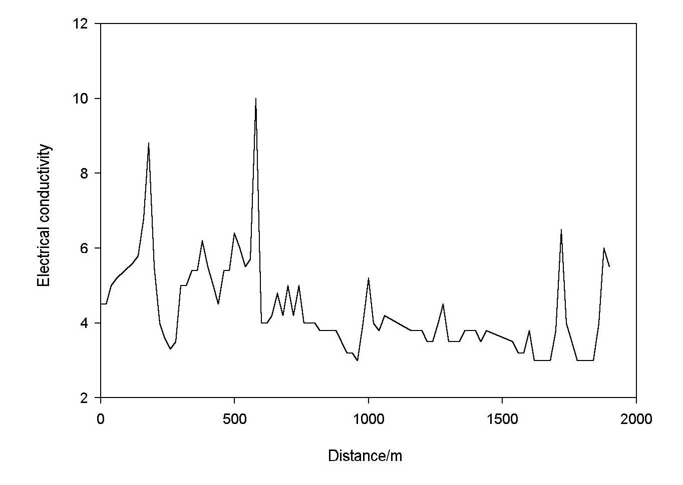
Figure 15. Graph of conductivities plotted against sampling position along the transect near to Biggin, Derbyshire (England).

Table 5 gives the summary statistics of the conductivity measurements that were transformed to logarithms before computing the variogram because of the large skewness value. The variogram of the transformed conductivity measurements, Figure 16, suggests that the variation is periodic as was the case for the radon concentrations. A periodic model with a power function, Equation (16), fitted the best: it has a wavelength of 182.6 m, which is shorter than that of radon (Table 6). The variogram of the slope angle, Figure 17, was fitted by a periodic function with power function. It has a wavelength of 171.4 m which is close to that of conductivity, Table 6. The slope angle possibly reflects weak terracing along the transect that might be associated with the major joint pattern in the Carboniferous limestone. The relation between the wavelength of about 175 m and the major joint spacing in the Carboniferous limestone needs to be explored further.

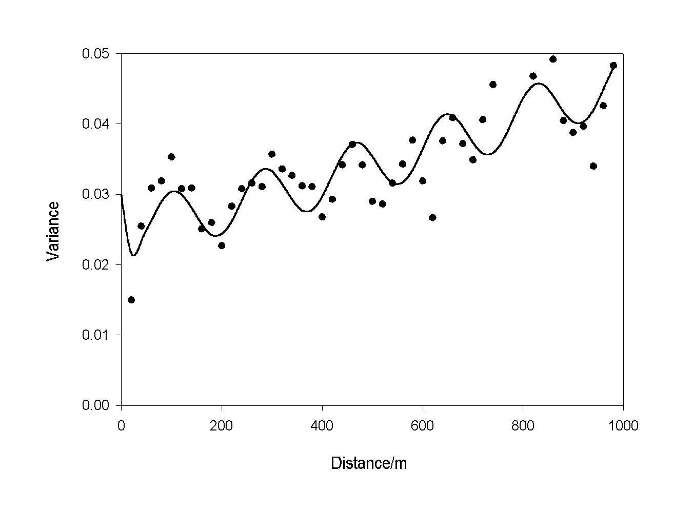
Figure 16. Variogram of conductivities for the transect near to Biggin, Derbyshire: the symbols are the experimental semivariances and the solid line is the fitted model.

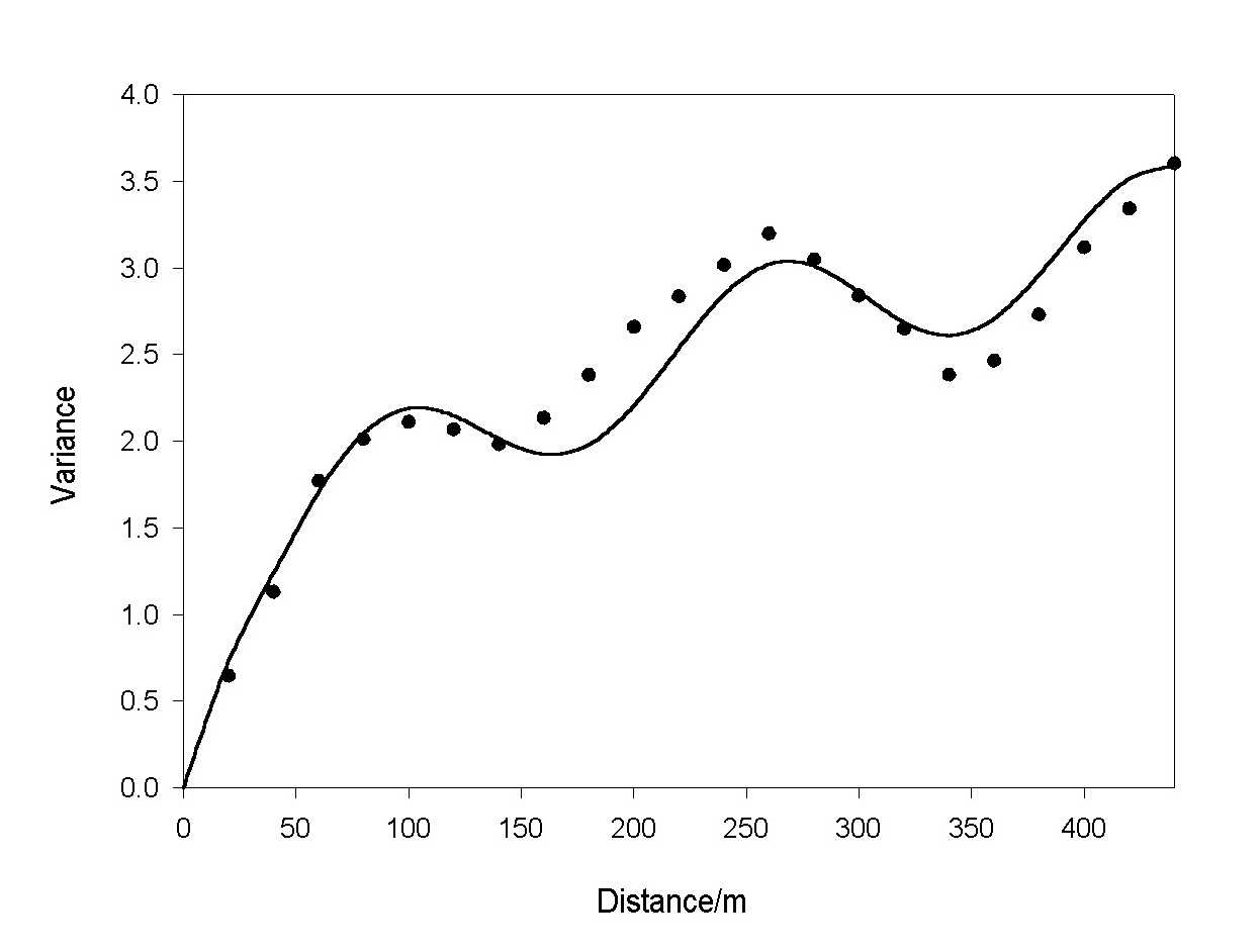
Figure 17. Variogram of slope angle for the transect near to Biggin, Derbyshire: the symbols are the experimental semivariances and the solid line is the fitted model.

Table 5. Summary statistics for the transect survey on a single lithology in Derbyshire

Table 6. Variogram model parameters for properties measured along the transect in Derbyshire.

5. Discussion and conclusion

To establish meaningful correlations between radon concentration and radiation-related illnesses in specified regions, there is a need to know how radon varies spatially, i.e., its structure and scale. This should provide a basis for choosing an appropriate method of prediction and for designing a suitable sampling scheme. These considerations are vital when planning surveys of large areas because of the enormous costs involved. Reliable estimates of radon and of the risk of developing diseases is vital because of the implications for locating new houses, for building practices, and for ameliorating the effects of radon in existing properties.

Our results suggest that geology is the major factor controlling the spatially dependent component of the variation in soil radon concentration. This has been suggested by others such as Ball et al. (1991), but we have been able to quantify and illustrate this effect. Our results also show that radon varies locally in a very erratic fashion and this supports the findings of Reimer and Gundersen (1989) that homes only 100 m apart had radon values that differed by two orders of magnitude. The surveys described here also suggest that in some areas there might be a spatially correlated component in the variation as well as a locally erratic one remaining within the lithological units. This latter was reflected in the substantial nugget variance in the sample variograms of the second Buxton, survey and of the transect survey. For the nested survey near to Buxton when the effects of geology were removed, 53% of the variation in the residuals occurred within 4 m, nevertheless, there was evidence of spatially dependent variation over a much longer distance.

The survey in two dimensions on the single lithology showed that it was feasible to estimate radon values by kriging within the lithological units as Voltz and Webster (1990) suggested. The results of estimating and mapping radon concentration led us to explore the variation in elevation and particle size distribution, which appear to be related with it and with each other. The results of the transect survey suggest that the variation is soil depth is also related to that of radon, and this in turn might be associated with the underlying karst topography of the limestone. This requires further investigation.

The procedure that we recommend from our findings for estimating radon is to stratify the area on the basis of lithology first, and then determine whether geology accounts for all of the spatially dependent variation using the variogram of the raw data and that of the residuals. If so sampling should then be optimized to estimate the mean radon concentration within the geological units reliably. If there is spatial dependence remaining within the classes then sampling should be optimized for kriging. This will provide reliable estimates of radon concentration with known error within strata.

Acknowledgments

The author thanks Professor R. Webster for the use of software, and Dr. S.A. Durrani for advice on radon monitoring.

References

Agard, S.S. and L.C.S. Gundersen, 1991. The geology and geochemistry of soils in Boyertown and Easton, PA, in L.C.S. Gundersen and R.B. Wanty, Eds. Field Studies of Radon in Rocks, U.S. Geological Survey Bulletin 1971, pp. 51-63.

Aitkenhead, N., J.I. Chisholm and I.P. Stevenson, 1985. Memoir for 1:50 000 geological sheet 111 (England and Wales) , British Geological Survey, HMSO, London, England.

Akerblom, G., P. Anderson and B. Clavensjo, 1984. Soil gas radon - A source for indoor radon daughters. Radiation Protection Dosimetry, 7, pp. 49-54.

Badr, I., M.A. Oliver, G.L. Hendry and S.A. Durrani, 1993. Determining the spatial scale of variation in soil radon values using a nested survey and analysis. Radiation Protection Dosimetry, 49, pp. 433-442.

Ball, T. K., R.A. Nicholson and D. Peachey, 1985. Gas geochemistry as an aid to detection of buried mineral deposits. Transactions of the Institute of Mining and Metallurgy, Section B, 94, pp. 181-188.

Ball, T.K., D.G. Cameron, T.B. Colman and P.D. Roberts, 1991. Behaviour of radon in the geological environment: a review. Quarterly Journal of Engineering Geology, 24, pp. 169-182.

Binks, K., 1989. Radon exposure and leukaemia (Letter to the Editor). The Lancet, ii, p. 562.

Bowie, C. and S.H.U. Bowie, 1991. Radon and health. The Lancet, 337, pp. 409-413.

Burgess, T.M. and R. Webster, 1984. Optimal sampling strategies for mapping soil types, I. Distribution of boundary spacings. Journal of Soil Science, 35, pp. 641-654.

Burrough, P.A., 1983. Multiscale sources of spatial variation in soil, II. A non- Brownian fractal model and its application. Journal of Soil Science, 34, pp. 599-620.

Clarke, R.H. and T.R.E. Southwood, 1989. Risks from ionising radiation. Nature, 338, pp. 197-198.

Durrani, S.A., N.A. Karamdoust, C.J.M. Griffiths and S.A.R. Al-Najjar, 1993. Radon measurements at the site of a former coal-burning station, in Sohrabi, M., Ahmed, J. V., and Durrani, S. A., eds., Proceedings of the International Conference on High Levels of Natural Radiation, (Ramsar, Iran), International Atomic Energy Agency, Vienna, pp. 207-220.

Duval, J.S. and J.K. Otton, 1990. Radium distribution and indoor radon in the Pacific Northwest. Geophysical Research Letters, 17, pp. 801-804.

Frost, D.V. and J.G.O. Smart, 1979. Memoir for 1:50 000 geological sheet 125 (England and Wales). Geological Survey of Great Britain, HMSO, London, England.

Green, B.M.R., P.R. Lomas and M.C. O'Riordan, 1992. Radon in Dwellings in England. National Radiological Protection Board NRPB-R254, HMSO, London, England.

Griffiths, C.J.M., 1989. Determination of radon activity concentrations in soils using solid state nuclear track detectors and the can technique. Unpublished Masters Thesis, University of Birmingham.

Henshaw, D.L., J.P. Eatough and R.B. Richardson, 1990. Radon as a causative factor in the induction of myeloid leukaemia and other cancers. The Lancet, 335, pp. 1,008-1,012.

Hung, I. F., C.C. Yu and C.J. Tung, 1994. Indoor radon concentrations in Taiwanese homes. Journal of Environmental Science and Health Part A - Environmental Science and Engineering, 29, pp. 1,859-1,870.

Jones, R.L., 1995. Soil uranium, basement radon and lung cancer in Illinois, USA. Environmental Geochemistry and Health, 17, pp. 21-24.

Journel, A.G. and C.J. Huijbregts, 1978. Mining Geostatistics, Academic Press, London, England.

Lucas, H.F., 1957. Improved low-level alpha scintillation counting for radon. Review Scientific Instruments, 68, pp. 680-683.

Lucie, N.P., 1989. Radon exposure and leukaemia (Letter to the Editor), The Lancet, ii, pp. 99-100.

Marcuse, S., 1949. Optimum allocation and variance components in nested sampling with an application to chemical analysis. Biometrics, 5, pp. 189-206.

Matheron, G., 1965. Les Variables Régionalisées et leur Estimation, Masson, Paris.

Matheron, G., 1971. The theory of regionalized variables and its applications. Cahiers du Centre de Morphologie Mathématique de Fontainebleau, no. 5, Ecole des Mines de Paris, (Fontainebleau).

McBratney, A. B., R. Webster and T.M. Burgess, 1981. The design of optimal sampling schemes for local estimation and mapping of regionalized variables, I. Theory and method. Computers and Geosciences, 7, pp. 331-334.

McNeill, J. D., 1980. Electromagnetic terrain conductivity measurement at low induction numbers. Geonics Limited Technical Note Tn-6, pp. 1-6.

Miesch, A.T., 1975. Variograms and variance components in geochemistry and ore evaluation, in Whitten, E. H. T., Ed., Quantitative studies in the geological sciences, Geological Society of America, Memoir/I, 142 pp. 333-340.

Miles, J.C.H. and M. Olast, 1989. Results of the 1989 CEC intercomparison of radon detectors. National Radiological Protection Board, HMSO, London, U.K.

National Radiological Protection Board, 1992. Documents of the NRPB, Vol. 1, No. 1, Her Majesty's Stationery Office (HMSO), London, U.K.

Nero, A.V., A.J. Gadgil, W.W. Nazaroff and K.L. Revzen, 1990. Indoor Radon and Decay Products: Concentrations Causes, and Control Strategies. DOE/ER-0480P, Department of Energy, Office of Health and Environmental Research, Washington, D.C.

O'Connor, P.J., V. Gallagher, G. Van den Boom, G., Hagengorf, et al., 1992. Mapping of Rn-222 and He-4 in soil gas over a karstic limestone-granite boundary: Correlation of high indoor Rn-222 with zones of enhanced permeability. Radiation Protection Dosimetry, 45, pp. 215-218.

Oliver, M.A., K.R. Muir, R. Webster, S.E. Parkes, A.H. Cameron, M.C.G. Stevens and J.R. Mann, 1992. A geostatistical approach to the analysis of pattern in rare disease. Journal of Public Health Medicine, 14, pp. 280-289.

Oliver, M.A., and R. Webster, 1986. Combining nested and linear sampling for determining the scale and form of spatial variation of regionalized variables. Geographical Analysis, 18, pp. 227-242.

Oliver, M.A. and R. Webster, 1987. The elucidation of soil pattern in the Wyre Forest of the West Midlands, England. II. Spatial distribution. Journal of Soil Science, 38, pp. 293-307.

Peake, R.T. and C.T. Hess, 1987. Radon and geology: some observations. In: D. D. Hemphill, Ed., Trace Substances in Environmental Health--XXI. Proceedings of the 21st Annual Conference, University of Missouri, Columbia, MO, pp. 186-194.

Reimer, G. M., 1991. Derivation of radon migration rates in the superficial environment by the use of helium injection experiments. In: Gundersen, L.C.S., and Wanty, R.B., Eds., Field studies of radon in rocks, soil and water, U.S. Geological Survey Bulletin 1971, pp. 33-38.

Reimer, G.M. and L.S. Gundersen, 1989. A direct correlation among indoor Rn, and soil gas Rn and geology in the Reading Prong near Boyertown, Pennsylvania. Health Physics, 57, pp. 155-160.

Reimer, G.M., L.C.S. Gundersen, S.L. Szarzi and J.M. Been, 1991. Reconnaissance approach to using geology and soil-gas radon concentrations for making rapid and preliminary estimates of indoor radon potential. in Gundersen, L. C. S., and Wanty, R. B., Eds., Field studies of radon in rocks, soil and water, U.S. Geological Survey Bulletin 1971, pp. 177-181.

Ross, G.J.S., 1987. Maximum likelihood program, Numerical Algorithms Group, Oxford, England.

Swedjemark, G. A., 1986. Swedish limitation schemes to decrease Rn daughters in indoor air. Health Physics, 51, pp. 569-578.

Voltz, M. and R. Webster, 1990. A comparison of kriging, cubic splines and classification for predicting soil properties from sample information. Journal of Soil Science, 41, pp. 473-490.

Webster, R. and B. Boag, 1992. A geostatistical analysis of cyst nematodes in soil. Journal of Soil Science, 43, pp. 583-595.

Webster, R. and C.H.E. de la Cuanalo, 1975. Soil transect correlograms of North Oxfordshire and their interpretation. Journal of Soil Science, 26, pp. 176-194.

Webster, R., and M.A. Oliver, 1990. Statistical Methods for Soil and Land Resource Surveys, Oxford University Press, Oxford, England.

Youden, W.J. and A. Mehlich, 1937. Selection of efficient methods for soil sampling. Contributions of the Boyce Thompson Institute of Plant Research, 9, pp. 59-72.