Return to GeoComputation 99 Index
David Kidner1, Mark Dorey1 & Derek Smith2
University of Glamorgan
1School of Computing
2Division of Mathematics & Computing
Pontypridd, Rhondda Cynon Taff
WALES, U.K. CF37 1DL
E-mail:dbkidner@glam.ac.uk
This paper advocates the use of more sophisticated approaches to the mathematical modelling of elevation samples for applications that rely on interpolation and extrapolation. The computational efficiency of simple, linear algorithms is no longer an excuse to hide behind with today's advances in processor performance. The limitations of current algorithms are illustrated for a number of applications, ranging from visibility analysis to data compression.
A regular grid digital elevation model (DEM) represents the heights at discrete samples of a continuous surface. As such, there is not a direct topological relationship between points; however, for a variety of reasons, users consider these elevations to lie at the vertices of a regular grid, thus imposing an implicit representation of surface form. For most GIS, a linear relationship between 'vertices' is assumed, while a bilinear representation is assumed within each DEM 'cell'. The consequences of imposing such assumptions can be critical for those applications that interpolate unsampled points from the DEM. The first part of the paper demonstrates the problems of interpolation within a DEM and evaluates a variety of alternative approaches such as bi-quadratic, cubic, and quintic polynomials and splines that attempt to derive the shape of the surface at interpolated points.
Extrapolation is an extension of interpolation to locations outside the current spatial domain. One can think of extrapolation as "standing in the terrain and given my field of view, what is my elevation at a location one step backwards?" This approach to elevation prediction is at the heart of many new techniques of data compression that are applied to DEMs. The demand for better data compression algorithms is a consequence of finer resolution data, e.g. LiDAR, and the wider dissemination of DEMs by intranet and internet. In a similar manner to the interpolation algorithms, the basis of elevation prediction is to determine the local surface form by correlating values within the 'field of view'. The extent of this field of view can be the nearest three DEM vertices that are used to bilinearly determine the next vertex. The second part of the paper evaluates this approach for more extensive fields of view, using both linear and non-linear techniques.
Applications of digital terrain modelling abound in civil engineering, landscape planning, military planning, aircraft simulation, radiocommunications planning, visibility analysis, hydrological modelling, and more traditional cartographic applications, such as the production of contour, hill-shaded, slope and aspect maps. In all such applications, the fundamental requirement of the digital elevation model (DEM) is to represent the terrain surface such that elevations can be retrieved for any given location. As it is often unlikely that the sampled locations will coincide with the user's queried locations, elevations must be interpolated from the DEM. To date, most GIS applications only consider linear or bilinear interpolation as a means of estimating elevations from a regular grid DEM. This is due mainly to their simplicity and efficiency in what may be a time-consuming operation, such as a viewshed calculation; however, some researchers have recently focused attention on the issue of error in digital terrain modelling applications, particularly for visibility analysis. To this extent, this paper examines the choice of interpolation technique within a regular grid DEM, in terms of producing the most suitable solution with respect to accuracy, computational efficiency, and smoothness.
The regular grid DEM data structure is comprised of a 2-D matrix of elevations, sampled at regular intervals in both the x and y planes. Theoretically, the resolution or density of measurements required to obtain a specified accuracy should be dependent on the variability of each terrain surface. The point density must be high enough to capture the smallest terrain features, yet not too fine so as to grossly over-sample the surface, in which case there will be unnecessary data redundancy in certain areas (Petrie, 1990). The term regular grid DEM suggests that there is a formal topological structure to the elevation data. In reality, the DEM is only representative of discrete points in the x, y planes (Figure 1) and should not be thought of as a continuous surface (Figure 2); however, it is often perceived as such when combined with a method of surface interpolation, such as a linear algorithm.

Figure 1 - Two Views of a DEM as a Set of Independent Discrete Elevation Samples and as a Constrained Topological Grid of Elevations With an Implicit Linear Surface Over the Grid "Cells"
We should not be constrained to thinking of interpolation within an (imaginary) grid cell, but rather of interpolation within a locally defined mathematical surface that fits our discrete samples - the extent and smoothness of which is related to the application and requirements of the user. Leberl (1973) recognised that the performance of a DEM depends on the terrain itself, on the measuring pattern and point density in digitising the terrain surface, and on the method of interpolating a new point from the measurements. In the meantime, many researchers have focused on the relationship between sampling density and the geomorphology and characterisation of terrain surfaces; however, the subject of interpolation has largely been ignored. It is our belief, that users should be aware of the limitations of linear interpolation or any other technique that restricts the surface function to just the vertices of the grid cell. In many instances, linear techniques can produce a diverse range of solutions for the same interpolated point. A higher order interpolant that takes acount of the neighbouring vertices, either directly or indirectly as slope estimates, will always produce a better estimate than the worst of these linear algorithms. The paper will demonstrate that by extending the local neighbourhood of vertices used in the interpolation process, accuracy will improve. For many applications such as visibility analysis or radio path loss estimation, very small elevation errors may propagate through to large application areas. Perhaps one of the key discussion areas with respect to higher order interpolation, is what is the ideal or optimal range of neighbourhood elevations that should be used in the interpolation process?
The interpolation problem can be extended into one of extrapolation, in which we estimate elevations outside the domain of the current range of elevations. Again, it is easy to demonstrate that by extending the local neighbourhood of elevation samples, better estimates can be extrapolated or predicted. Extrapolation is currently a hot topic of research within the fields of data and image compression. Data compression can be simply defined as the removal of the redundancy which a data set inherently possesses. To this extent, some researchers have investigated the use of image compression algorithms for DEMs (Franklin, 1995). In the case of DEMs, most of the inherent redundancy is due to the correlation between neighbouring elevations and the use of fixed-size word lengths, such as a 2-byte integer (Kidner & Smith, 1992). Most researchers who have attempted to compress DEMs, recognise these properties, and have adopted a two-stage strategy that decorrelates the DEM (via extrapolation or prediction), and then stores the corrections to these elevations using a data compression algorithm. The paper illustrates how such a simple, lossless technique can reduce the storage overheads of DEMs by 85% to 90%, or 40% to 60% better than GZIP.
For both interpolation and extrapolation we will show that extending the DEM neighbourhoods for these types of operations will yield better results, whether it be for determining intervisibility or efficiently storing DEMs. Another issue that is addressed is the extent of these neighbourhoods. As terrain may exhibit general trends as well as very local fluctuations, or low and high frequency components, it is important to consider the optimal range of vertices, at which point performance might start to tail-off or deteriorate.
Bearing in mind that a DEM represents a sample of elevations at specific locations, we need to consider how we can estimate or retrieve heights for other locations. Consider a set of four vertices forming a grid square, with an interpolating profile passing through the DEM as illustrated below in Figure 2. We are faced with a number of interpolation scenarios, with the most popular being that of linear interpolation along the boundaries of the grid cell at points A and B; hence,
A = 50 + 0.2(72-50) = 54.4, and
B = 54 + 0.4(72-54) = 61.2.
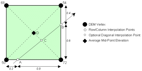
Figure 2 - Profile Interpolation through a Square Cell of a Regular Grid DEM
While these are useful estimates for our profile, we may have missed some important features within the grid cell. For example, what if the NW-SE diagonal is representative of a ridge line (Figure 3a)? The profile will ignore the local maximum, which could be a critical point in the line-of-sight evaluation. On the other hand, the NE-SW diagonal may be representative of a channel (Figure 3b), in which case our initial row and column interpolations are sufficient. More general interpolation problems may be to determine where the 60 metre contour passes through the grid cell of Figure 2, or simply to evaluate the elevation of D. We can now see that it is important to use as much information as possible in reconstructing the cross-section including, for example, the intersecting diagonal of each grid cell (i.e., point C in Figure 2), in addition to the row and column intersections. In effect, a profile will always pass through two triangles of a grid cell, as opposed to our initial view of the one triangle formed by the intersected row and column. We are left with the question as to which approach is the correct one, if any? The linearly interpolated point at C along the NW-SE diagonal of Figure 1 will give us a value approaching 71 metres, compared to a value of approximately 58 metres on our original profile. Given only the information presented to us in Figure 2, we cannot determine which of these two approaches is the better. Both algorithms are equally valid or equally invalid. They both assume a triangular lattice exists between DEM elevations, where the triangle faces approximate constant slope. Conveniently, these linear constraints either maximise or minimise the number of interpolations. As such, for both algorithms an arbitrary decision has been made in each and every grid cell about the existence of a linear feature, which may or may not exist in the real world. This is guaranteed to create anomalies in the reconstructed profiles, as ridges may be modelled as orthogonal channels and vice versa. There are a number of compromise solutions that attempt to average out these arbitrary minimum and maximum results, the simplest of which is a bilinear surface (Figure 3c) and described in Section 3. The profile through the grid cell of Figure 2 is illustrated below in Figure 3 for each of these approaches. The cross sections clearly illustrate that the method of profile interpolation can give rise to serious concern. The problem is extended further into an intervisibility calculation in Figure 4, which clearly demonstrates that these interpolation errors may propagate through to large application errors.
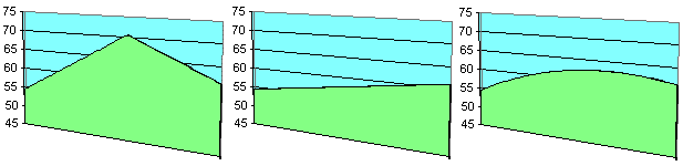
Figure 3 - Profile (Cross-Section) Interpolation through Points A to B in the Grid Cell of Figure 2
(a) NW-SE Ridge (b) NE-SW Channel (c) Bilinear Surface
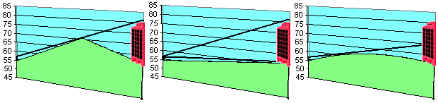
Figure 4 - Visibility of a 20 m Building at B Viewed at a Height of 1.75 m above A in the Grid Cell of Figure 2
(a) NW-SE Ridge - Obscured (b) NE-SW Channel - Visible (c) Bilinear Surface - Partially Visible
The determination of a surface defined by regularly or irregularly spaced data has been stated by Schumaker (1976) as:
"Given the points (xi , yi , zi ), for i = 1, 2, …, n, over some domain, a function z = f(x, y) is desired which reproduces the given points, and produces a reasonable estimate of the surface (z) at all other points (x, y) in the given domain"
There are a variety of possible interpolation procedures presented in the literature, some of which are described in the context of interpolation for a DEM (Lerberl, 1973; Schut, 1976; Crain, 1970; Rhind, 1975; Davis et al., 1982; and Petrie & Kennie, 1987). Lerberl (1973) suggests that the choice of an interpolation procedure is made on the basis of intuition, logical considerations and experience; however, we require a more systematic and proven choice of algorithm.
The most commonly used interpolation method for a regular grid DEM is patchwise polynomial interpolation. The general form of this equation for surface representation is:
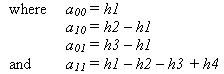
where hi is the height of an individual point i, x and y are its rectangular coordinates of i, and a00, a10, a01, …, amn are the coefficients of the polynomial. Since the coordinates of each vertex are known, the values of the polynomial coefficients can be determined from the set of simultaneous equations that are set up, one for each point. For any given point with known coordinates x, y, the corresponding elevation can be determined by a substitution into this equation.
In essence, most interpolation techniques can be related to various terms of the equation in [1]. This suggests that there may only be a limited number of strategies that can possibly be chosen for interpolation. While this might be true for the number of unique polynomial equations, there also are a plethora of different approaches for determining the coefficients a of these equations. The different strategies are outlined briefly below, while Section 4 will consider issues such as derivative estimation.
This is by far the simplest and crudest approach for interpolation, and yet can still be found in some modelling packages. The level plane takes the form of:
where a00 may be the height of the closest DEM vertex (nearest neighbour), or alternatively, it may be taken as the arithmetic mean of the four surrounding vertices of the grid cell. The result is a discontinuous representation of the terrain by a set of level surfaces of different heights, in a similar manner to the steps of Figure 1.
The linear plane is a three-term polynomial of the form:
formed by fitting a triangle to the three closest DEM vertices. Surface fitting by plane triangles was popular in many early DTM systems (Leberl, 1973), but has been largely superseded by the more popular bilinear interpolation. Linear plane interpolation is more likely to be used in triangulated irregular networks (TINs) that have been derived from a regular grid DEM with little or no vertex removal.
The choice of grid cell diagonal in the representation of the linear plane is quite arbitrary, which can possibly result in significant differences in interpolated elevations. Double linear interpolation attempts to minimise the likelihood of such errors by averaging the linear plane heights of the two triangles into which a grid cell can be divided by one of its diagonals. It has been described as computing the height of the point at the centre of the grid cell as the mean of the heights of the four corner vertices, followed by linear interpolation in each of the four triangles formed by the sides and two diagonals (Schut, 1976).
The concept of linear interpolation between two points can be extended to bilinear interpolation within the grid cell. The function is said to be linear in each variable when the other is held fixed. For example, to determine the height hi at x, y in Figure 5, the elevations at y on the vertical boundaries of the grid cell can be linearly interpolated between h1 and h3 at ha, and h2 and h4 at hb. Finally, the required elevation at x can be linearly interpolated between ha and hb.
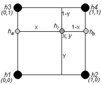
Figure 5 - Unit Square Grid Cell Layout for Bilinear Interpolation
The bilinear function is akin to fitting a hyperbolic paraboloid to the four vertices of the grid cell. It is usually written as:
By considering quadratic terms of [1], we arrive at the nine-term biquadratic function:
Occasionally, the x2y2 term is omitted, such that an 8-term biquadratic function of the form:
is advocated by some commentators (Schut, 1976). In both cases, we need to determine which vertices are to be used to formulate these equations. The simplest approach is to make the local surface fit the elevations at the corners of the grid cell in which we wish to interpolate, and also at the middle of the sides of the grid element (Figure 6). If the 9-term biquadratic of [5] is favoured, the additional ninth point is an estimate at the centre of the grid cell. The heights in the middle of each grid cell side can be calculated using a cubic polynomial or spline through the nearest four row or column vertices.
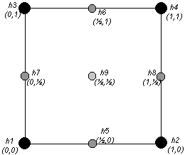
Figure 6 - Biquadratic Surface Patch Configuration of DEM Vertices and Estimates
A true biquadratic polynomial should be applied to a local set of 3 by 3 elevation vertices, rather than the approach of 3.5; however, as this covers 2 by 2 grid cells, then for each point to be interpolated, there are four possible biquadratic surfaces to be considered over 4 by 4 vertices (Jancaitis and Junkins, 1973). Using a function of the form [5], the four interpolations are unlikely to be the same, so a weighted average needs to be calculated, which takes account of the distance of the point from the origin of the cell. Jancaitis suggests a weight function of the general form:
which is of the third order in both x and y. With the second order biquadratic functions, the resulting surface is of the fifth order in both x and y over the central grid cell, thus ensuring smoothness as well as continuity.
In Section 3.4 and Figure 5, it was shown how 1-D piecewise linear interpolation could be used to interpolate values in the 2-D plane. This can be extended into piecewise cubic interpolation using a polynomial of the form:
With this function, we require four values to solve the coefficients. If the side of the grid cell is assumed to lie between 0 and 1, the function and its differential can be evaluated at these end-points; hence, we also require estimates of slope at the two end-points or DEM vertices. In the simplest case, slope can be estimated from the vertex either side of the end-point, as a simple gradient calculation (i.e., elevation change with respect to distance); thus, for any interpolation, we require the neighbouring 4 by 4 vertices of the central grid cell in which the point lies. Four interpolations are made in one direction, which then feed into a final interpolation in the orthogonal direction. Monro (1982) presents a simple algorithm for piecewise cubic interpolation, specifically for interpolating a denser grid of values from a sparser grid. In our study, we extended the slope estimation to two vertices either side of the end-points, thus resulting in a 6 by 6 neighbourhood of DEM vertices for each interpolation within a cell.
After bilinear interpolation, perhaps the most widely used technique is that of bicubic interpolation, certainly by computational geometers, if not GIS users. This makes use of the 16-term function:
Bicubic interpolation is the lowest order 2-D interpolation procedure that maintains the continuity of the function and its first derivatives (both normal and tangential) across cell boundaries (Russell, 1995). As we want the function to be valid over the grid cell of the interpolated point, we need to consider which 16 values to use to derive the coefficients. The common approach is to use the height at the four vertices, together with three derivatives at each vertex. The first derivatives h'x and h'y express the slope of the surface in the x and y directions, while the second (cross) derivative h''xy represents the slope in both x and y. In terms of solving the coefficients of [9], these values can be expressed by differentiating the x and y vectors independently, and then consecutively. For each of the vertices of the grid cell, the local coordinates (at 0,0, 1,0, 0,1 and 1,1) can be input into these equations to generate the 16 equations to solve [9]. Press et al., (1988) present algorithms for piecewise cubic, bicubic polynomial and bicubic spline interpolation. Methods for determining the slope estimates or partial derivatives are presented in Section 3.10.
A simpler approach described by Schut (1976) is to use the 12-term incomplete bicubic polynomial:
In this instance the cross-derivative h''xy is not required, leaving the four corner elevations and eight first-order derivatives sufficient to compute the parameters. While the total surface is continuous, it is only smooth at the nodes.
The simplest function that ensures smoothness of the first derivatives across the grid cell boundaries is biquintic interpolation. This makes use of the 36-term function:
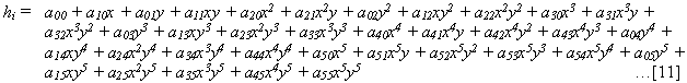
It is evaluated in exactly the same way as bicubic interpolation, but for each of the four vertices of the grid cell, we now require nine values. These are the elevations themselves, and the derivatives h'x, h'y, h''xx, h''xy, h''yy, h'''xxy, h'''xyy and h''''xxyy. By substituting the local coordinates of the four vertices, we can solve the resulting 36 equations, or re-write in terms of the coefficients of [11].
For some of the latter interpolation techniques described above, various derivatives of the functions at the four corners of the DEM cell need to be approximated from the elevations. As Press et al. (1988) point out "it is important to understand that nothing in the equations requires you to specify the derivatives correctly." The better the approximation, the better the performance of the interpolation. There are a variety of implementations of algorithms, such as the bicubic interpolating polynomial, due to the approach used to estimate these derivatives. The lower order derivative approximations can be found in many texts on numerical algorithms or finite elements, but the derivation of the mixed and higher order derivatives is less well documented. One exception is Russell (1995) who presents a variety of approaches for up to the eight derivatives of the biquintic polynomial. Akima (1974a, 1974b, 1996) also presents less conventional approaches for estimating the derivatives h'x, h'y and h''xy for bicubic interpolation.
In order to evaluate the performance of the various algorithms, it is essential to have confidence in the quality of the data. A common approach is to use a set of test functions that represent a variety of different phenomena. Franke (1979) and Akima (1996) use six mathematical surface functions (illustrated below in Figure 7), that are used to determine the values on uniform grids, which in turn are used to interpolate denser grids. The performance of the interpolation algorithms can then be evaluated for these denser grids against the surface function values.
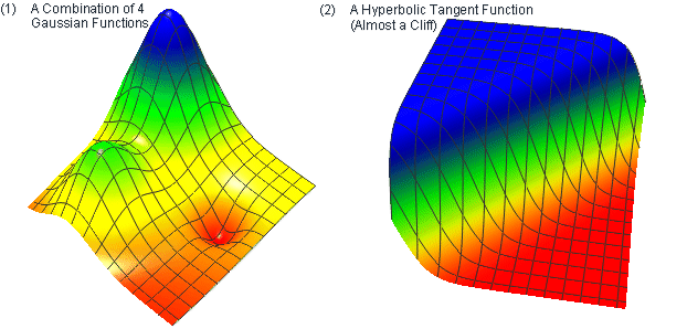
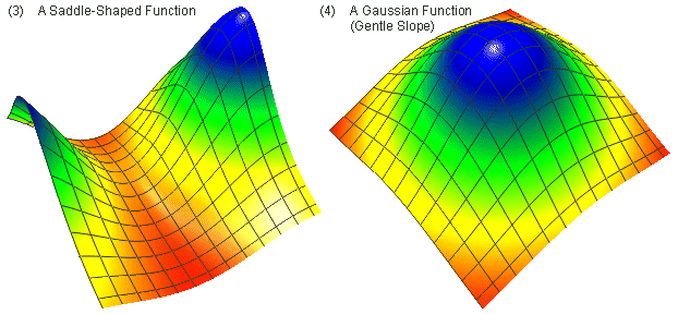
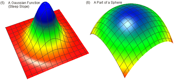
Figure 7 - The Six Mathematical Test Functions of Franke (1979) & Akima (1996)
In total, we implemented more than forty different interpolation algorithms, many of which utilised the same methodology, but different approaches for estimating the derivatives (e.g. for bicubic and biquintic interpolation) or different mid-point estimates (e.g., for biquadratic interpolation). The best performing algorithm in each category is presented in the results below. These algorithms include the level plane, the two linear planes defined by the diagonal, double linear interpolation, bilinear interpolation, the 8-term and 9-term biquadratic function, the Jancaitis 5th order weighted biquadratic surfaces, piecewise cubics, 12-term and 16-term bicubic functions using text-book derivative estimates alongside Akima's (1996) derivatives, and finally biquintic interpolation. The algorithms were tested on a number of sparse grids to interpolate denser grids. Performances were evaluated and ranked on the basis of error variance. Table 1 presents the rankings of each of these algorithms for each of the surface functions of Figure 7. Overall ranking was adjudged by summing the individual rankings.
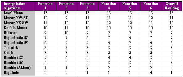
Table 1 - Ranking of Interpolation Algorithms with Respect to Test Functions of Figure 7
Rank correlation coefficients were calculated on a pairwise basis for each set of rankings, and between the overall and individual rankings. These results and visual inspection of Table 1 demonstrate strong correlation between the individual results.
The results demonstrate that higher order interpolation will always produce better results than linear interpolation algorithms, while the best overall results were achieved using the 36-term biquintic algorithm. Somewhat surprising was the disappointing performance of the weighted biquadratic functions; however, on tests with actual terrain at multiple scales (or DEM resolutions), the Jancaitis algorithm performed better. In these tests, it was more difficult to distinguish between the rankings of the Jancaitis and higher-order functions.
In recent years there has been increased activity in lossless data compression, particularly applied to images, and just as importantly, spatial data. With the advances in spatial data acquisition, particularly in remote sensing, users do not want to discard this finer resolution data. If the time, money, and effort have been put into the development of these products, then users need to be able to exploit the true potential of the data, without error. Lossy techniques will introduce error that may propagate through to larger application errors (e.g. for LiDAR DEMs). For an increasing number of users, this is unacceptable. It should be remembered that data compression is important for the efficient dissemination and communication of spatial data, particularly over networks, not just for efficient file storage.
Of the various techniques available, predictive or extrapolation techniques are perhaps the simplest and most efficient. With respect to terrain data, the DEM is processed vertex by vertex in raster order, with the current vertex extrapolated from the previous vertices. Providing that the receiving user is aware of the prediction algorithm used, then only the extrapolation error correction needs to be encoded. If the extrapolation is reasonably accurate, then the distribution of prediction errors will be concentrated near zero and will have a significantly lower zero-order entropy than the original image (Figure 8).
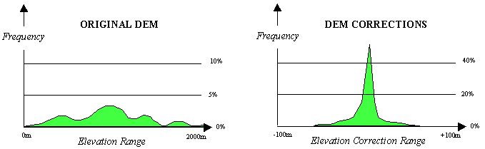
Figure 8 - Typical Frequency Distribution of DEM Heights Before and After Extrapolation
DEM elevation values themselves do not necessarily represent information rates. Instead, the average information rate is given by the entropy, which can be thought of as the efficiency of the extrapolation or decorrelation step. It is more generically defined as the average number of bits required to represent each symbol of a source alphabet, which in our case are the prediction error corrections. Entropy is defined as:
where pi is the probability of each of the unique elevation corrections. This also is called the zeroth-order entropy, since no consideration is given to the fact that a given sample may have statistical dependence on its neighbouring elevations; hence, the better we can model or predict terrain, then the lower the entropy will be, hopefully resulting in higher compression ratios. The error corrections can then be encoded using any of the traditional variable-length entropy coding techniques, such as Huffman coding or Arithmetic coding. Alternatively, the users' favoured data compression software can be used, such as WinZip, GZip, Compress, etc. The whole procedure for lossless DEM compression is illustrated in Figure 9.
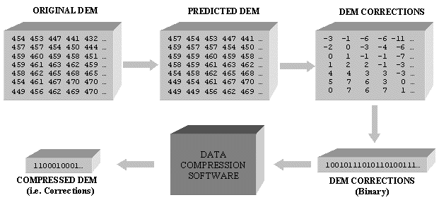
Figure 9 - Methodology for Lossless DEM Compression
In essence, we can consider the DEM compression problem to be one of identifying a suitable extrapolation algorithm to transform the frequency distribution of elevations into a more suitable distribution for statistical encoding. Such an approach has the potential to offer vast storage savings for very little programming or processing effort; however, higher compression ratios can be attained with the use of more sophisticated pre-processing algorithms.
The terrain predictor can be any function of a number of local elevations. Traditional interpolation algorithms that worked well in the tests above, are generally quite poor when it comes to extrapolation, or interpolation outside the current domain. More specifically, for the higher order functions, the errors can be a lot greater than using simple linear functions. This is due to the volatility of the polynomials such as cubics and quintics outside the modelled domain, resulting in errors that may increase by a factor of three, five, or the largest power of the algorithm.
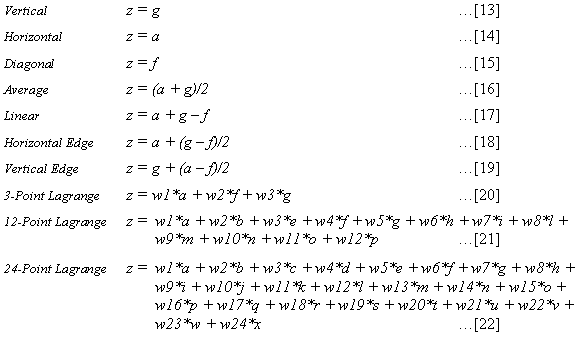
The predictor does not have to be very complex. In fact, some of the best predictors are often the simplest. In the simplest case, the next DEM vertex could be predicted as being the value of the previously encountered vertex. The JPEG lossless standard (Memon & Wu, 1997) uses a variety of such simple algorithms for image compression, which also can be applied to DEMs. In all cases, the predicted value is a linear weighted combination of vertices. Figure 10 illustrates the neighbourhood templates of vertices that we will consider in the prediction algorithms.
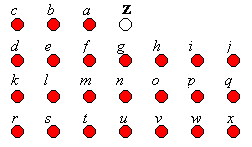
Figure 10 - Template Layout for the Various Algorithms for Predicting Point Z
In terms of actual algorithms, equations [13] to [22] outline the patterns, and where applicable, the weights of the specific vertices used during extrapolation. Equations [13] to [19] were adopted in the first lossless JPEG standard (along with with the null predictor z = 0, which we have deliberately omitted). Some of the weights are intuitive, but Smith & Lewis (1994) demonstrated a simple technique for optimising the weights for any given terrain surface. As such, the coefficients or weights can be obtained by minimising the mean square prediction error (mse) and constraining the mean error to be zero. This can be achieved using the method of Lagrange multipliers or solving the Yule-Walker equations that are defined by these criteria. The weights are optimal in the sense of minimising the mse. Equations [20] to [22] represent three optimal (Lagrange) predictors using different ranges of DEM neighbourhoods. For the algorithms that require larger neighbourhoods of vertices (e.g., [21] and [22]), the initial row and column are extrapolated using the Vertical [13] or Horizontal [14] predictors, while intermediate rows and columns are extrapolated using the Linear [17] predictor.
Newer approaches to prediction (Memon & Wu, 1997) attempt to increase performance (or lower the entropy) by recognising more of the general characteristics or underlying trends of the surface. These include searching for horizontal and vertical gradients among the previously encountered vertices. These techniques are non-linear, since the weights attempt to adapt for the previously encountered trends, possibly by exaggerating the next encountered vertex. Other techniques attempt to model the context of the local surface around the next vertex. If these contexts, or relationships between neighbouring vertices, can be quantised into a set number of classes, a look-up table could possibly be used to guide or adapt the prediction algorithm. This approach can be extended further by considering more dynamic approaches to prediction, including the use of neural networks (Ware et al., 1997). Despite implementing a number of these different strategies, the results were not always as good as even the simplest predictors. For this study, we will only consider the algorithms presented above.
To illustrate the use of the predictors for reducing the entropy of the DEM, consider the test data set for South Wales, consisting of a 60 km by 40 km O.S. DEM sampled at a resolution of 50 m (Figure 11). This is a good example of a DEM, which exhibits significant data redundancy, in a number of different guises. Most evident is the large proportion of sea level values (nearly 40%), that could be reduced using an approach such as run-length encoding; however, despite this bias in the elevation frequency distribution, the overall entropy or information content is about 9 bpe, as the elevation range is 0 to 569 metres.
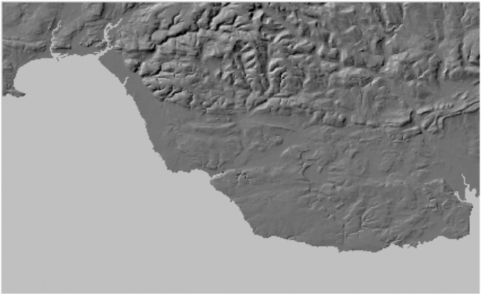
Figure 11 - 1201 by 801 Ordnance Survey 1:50,000 Scale DEM at 50m Resolution for South Wales
By applying the 24-point optimal (Lagrange) predictor to this DEM, the entropy reduces to under 2 bpe with only 74 unique elevation corrections. The distribution of these errors are illustrated below in Figures 12 and 13. The latter figure is viewed at a larger scale, so that the patterns of elevation corrections can be distinguished.
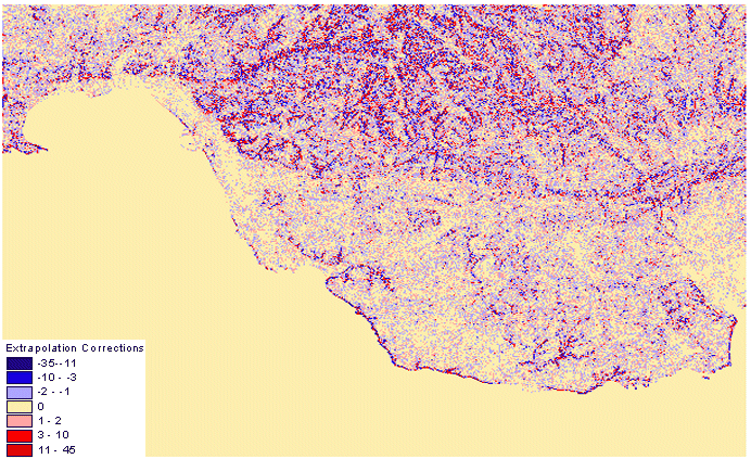
Figure 12 - 1201x801 Extrapolation Corrections for the 24-Point Lagrange Predictor
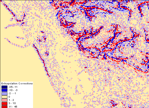
Figure 13 - Larger Scale View of the 24-Point Lagrange Predictor Corrections Demonstrating the Higher Level Correlation of Errors
Decorrelation involves prediction, and as the predictors are more nearly made to predict the future of the surface, the more the output from the decorrelator resembles random (or white) noise, however, Figure 13 demonstrates patterns in the predictor corrections that are far from random. These patterns correspond with geographical features such as cliffs, ridges, channels, and unexpected breaks in surface form. The ideal prediction algorithm must therefore be capable of recognising the smaller scale trends or specific geographic entities. Despite the reduction in entropy of about 7 bpe, there is still redundancy which some statistical data compression algorithms will not be able to exploit, as each individual data element is treated independently without any spatial awareness of local trends. An alternative is to use higher order statistical compression, that encodes a stream of data values. This will allow the actual compressed DEM to have an average code length less than the zero-order entropy. Table 2 below presents the results of the prediction algorithms outlined in Section 6 applied to the DEM of Figure 11.
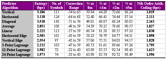
Table 2 - Results of the Extrapolation Algorithms for South Wales and Actual (Higher-Level) Compression
The results present the zeroth-order entropy of the prediction algorithms, the number of elevation corrections and its range, the percentage of DEM vertices that are predicted to within 0, 1, 2, and 5 metres, and the actual compressed code length using a higher order Arithmetic coding scheme. From this table, it can be deduced that the larger neighbourhoods of vertices that are used within the prediction process will produce better performance, but when large neighbourhoods are used (e.g., 24 points), the additional processing time does not necessarily warrant the very small improvements. The results also indicate that a poor predictor can be redeemed by a good higher order statistical encoding algorithm. For example, the vertical predictor performs worse than the linear predictor (by about 1 bpe), but after Arithmetic Coding, the results are better for the vertical predictor. In this instance, Arithmetic Coding uses row-wise data (in the x-plane) which when combined with the vertical predictor (in the y-plane) is equivalent to the linear (xy-plane) predictor. There is no doubt further room for improvement with respect to the use of dynamic predictors and the flexibility of statistical data compression algorithms exist; however, the result of under 1.6 bpe for this DEM represents a storage saving in excess of 90% over the traditional 2-byte integer, and is significantly better than the 4.164 bpe, which GZIP could only manage.
Digital terrain modelling is now accessible to a much larger user audience via the recent developments in desktop GIS (e.g., ArcView: 3-D and Spatial Analyst, MapInfo: Vertical Mapper); however, GIS has suffered in the past from limited modelling capabilities, or the use of algorithms that were adopted on the grounds of simplicity and computational efficiency, rather than accuracy of performance. While the 1990s have also seen increased user awareness of error modelling in GIS analysis, there is a danger that digital terrain modelling might also fall into the traps of the past. Users would appreciate a wider range of modelling functions to meet the requirments of their specific applications, rather than be constrained to one underlying algorithm of the GIS. A good example of this is interpolation. Users might require an interpolation algorithm to query the height of a specific location, contour a surface, determine a cross-section for an intervisibility calculation, or perform a viewshed calculation. This paper has shown that the choice of interpolation algorithm will clearly affect accuracy. A possible compromise is to offer users greater flexibility through a wider choice of algorithms, such that a biquintic algorithm could be chosen for individual height queries, a bicubic algorithm for a line-of-sight profile calculation, or a bilinear algorithm for a viewshed calculation.
The results for the interpolation algorithms suggest that higher order techniques will always outperform linear techniques. The trend (or slopes) of the surface are important for interpolation, since we should not be constrained to using the nearest 3 or 4 vertices of the DEM cell. As a minimum, we would stipulate that a bicubic interpolation algorithm should be considered for mainstream DEM analysis. The arguments in the past of the computational efficiency of such algorithms have been superseded by recent technological developments in processor speeds. Users would only notice the increased overheads of derivative calculations for extensive operations such as large viewshed calculations.
While desktop GIS has brought digital terrain modelling to a larger audience, users face a bottleneck in the dissemination of DEMs by internet and intranet. Spatial data compression algorithms have a big part to play in the future of GIS. By extending the concepts of interpolation into extrapolation, we have presented some simple mathematical modelling approaches to DEMs that are error-free and can offer storage savings in excess of 90%. More dynamic modelling strategies are possible, which offer further room for improvement, and could be applied to other remotely sensed spatial data.
Akima, H. (1974a) "A Method of Bivariate Interpolation and Fitting Based on Smooth Local Procedures", Communications of the ACM, Vol.17, No.1, January, pp.18-20.
Akima, H. (1974b) "Bivariate Interpolation and Smooth Surface Fitting Based on Local Procedures", Communications of the ACM, Vol.17, No.1, January, pp.26-31.
Akima, H. (1996) "Algorithm 760: Rectangular-Grid Data Surface Fitting that has the Accuracy of a Bicubic Polynomial", ACM Transactions on Mathematical Software, Vol. 22, No. 3, pp. 357-361.
Crain, I.K. (1970) "Computer Interpolation and Contouring of Two-Dimensional Data: A Review", Geoexploration, Vol.8, pp.71-86.
Davis, D.M., J. Downing & S. Zoraster (1982) Algorithms for Digital Terrain Data Modeling, Technical Report DAAK70-80-C-0248, U.S. Army Engineer Topographic Laboratories, Fort Belvoir, Virginia.
Franke, R. (1979) A Critical Comparison of Some Methods for Interpolation of Scattered Data, Technical Report NPS-53-79-003, Naval Postgraduate School, Monterey, California.
Franklin, W.R. (1995) "Compressing Elevation Data", in Advances in Spatial Databases: Lecture Notes in Computer Science 951, Proc. of the 4th Int. Symp. on Large Spatial Databases (SSD'95), Portland, August, Springer.
Jancaitis, J.R. & J.L. Junkins (1973) Mathematical Techniques for Automated Cartography, Technical Report DAAK02-72-C-0256, U.S. Army Engineer Topographic Laboratories, Fort Belvoir, Virginia.
Kidner, D.B. & D.H. Smith (1992) "Compression of Digital Elevation Models by Huffman Coding", Computers & Geosciences, Vol.18, No.8, pp.1013-1034.
Kidner, D.B. & D.H. Smith (1998) "Storage-Efficient Techniques for Handling Terrain Data", Proc. of the 8th Int. Symp. on Spatial Data Handling (SDH'98), Vancouver, July.
Leberl, F. (1973) "Interpolation in Square Grid DTM", The ITC Journal.
Memon, N. & X. Wu (1997) "Recent Developments in Context-Based Predictive Techniques for Lossless Image Compression", The Computer Journal, Vol. 40, No. 2/3, pp. 127-136.
Monro, D.M. (1982) Fortran 77, Edward Arnold Publishers, London, pp. 209-212.
Petrie, G. & T.J.M. Kennie (1987) "Terrain Modelling in Surveying and Civil Engineering", Computer-Aided Design, Vol.19, No.4, May, pp.171-187.
Press, W.H., S.A. Teukolsky, W.T. Vetterling & B.P. Flannery (1988) Numerical Recipes (in C), Cambridge University Press.
Rhind, D. (1975) "A Skeletal Overview of Spatial Interpolation Techniques", Computer Applications, Vol.2, pp.293-309.
Russell, W.S. (1995) "Polynomial Interpolation Schemes for Internal Derivative Distributions on Structured Grids", Applied Numerical Mathematics, Vol. 17, pp. 129-171.
Schut, G.H. (1976) "Review of Interpolation Methods for Digital Terrain Models", Canadian Surveyor, Vol.30, No.5, December, pp.389-412.
Smith, D.H. & M. Lewis (1994) "Optimal Predictors for Compression of Digital Elevation Models", Computers & Geosciences, Vol. 20, No. 7/8, pp. 1137-1141.
Ware, J.A., O. Lewis & D.B. Kidner (1997) "A Neural Network Approach to the Compression of Digital Elevation Models", Proc. of the 5th GIS Research UK Conference (GISRUK'97), April, Leeds, pp. 143-149.