Return to GeoComputation 99 Index
Kevin Morris (1), David Hill (2) and Tony Moore (1)
1. Centre for Coastal and Marine Sciences, Plymouth Marine Laboratory, Plymouth, Devon, PL1 3DH United Kingdom
2. Institute of Hydrology, Crowmarsh Gifford, Oxfordshire, OX10 8BB United Kingdom
E-mail: K.Morris@ccms.ac.uk
Traditional geographical information systems (GISs) employ a two-dimensional or at best 2.5-dimensional framework, suitable for many applications. However, mapping the environment introduces certain problems not easily managed within existing systems. The natural environment is constantly changing and this requires a more dynamic way of handling such data. For instance, land-use may change from season to season or from year to year. Environmental media such as the oceans and the atmosphere, complicate matters further as processes that occur within them vary through three-dimensional space and through time.
In the past, time and depth have been handled as attributes to a feature. This can be very limiting, as there is no ready dimensional structure against which features can be displayed or manipulated relative to time and depth. In nearly all conventional GIS, the x and y dimensions alone are used to display spatial data in map form at any one time. This paper describes a GIS system that handles time or depth visualization of a feature in addition to mapping the feature horizontally. This treats time or depth as a dimension rather than an attribute, which is a prerequisite to effective multidimensional visualization and analysis (Raper and Livingstone 1995).
The STEM (Spatio-Time Environmental Mapper) has been developed for LOIS (Land-Ocean Interaction Study), a UK research project investigating features and processes in the coastal zone. STEM is a GIS data viewer fronting a database containing the highlights of LOIS.
STEM owes its flexibility to two key design objectives: a simple yet powerful query expression, retrieval and visualisation interface and secondly a generic database design that provides the core of the data-driven system. The database represents the real world in terms of objects (features) and properties (attributes). Features and attributes can vary in both space and time.
The natural world is an ever-changing environment. This change evolves from sub-second rates through to geological timescales and involves interactions between many environmental components including atmospheric, terrestrial, riverine, marine and geological. It is becoming increasingly important to understand the processes behind these changes in order that anthropogenic effects on the environment can be better managed (UNEP 1995). Central to this is the storage, access and visualization of all environmental data, to facilitate improved understanding of the data and better predictions through modelling (Peuquet and Qian 1997).
Traditionally, many environmental studies have concentrated on either local or broad-scale environmental patterns and processes over either relatively short or long timescales (Stafford et al. 1994). Such studies have also often concentrated on one environmental component. To understand the processes in the environment and to effect better management, it is now becoming more important to integrate all of these factors and provide a more holistic view of the environment (NERC 1994, UNEP 1995). Therefore, there is a requirement for this to be reflected within the software tools used to handle environmental data. Integrating the data and tools also avoids duplication of effort and provides a more cost-effective way of managing such data (Ehlers et al. 1990). Strebel et al. (1994) suggest that for environmental information systems to be of any real use, a major challenge is to integrate disparate data sets (collected with varying instrumentation / experiments of varying structure) and archive them effectively.
This paper describes a system developed to store, access and visualize environmental data using the four dimensions of x, y, z and time, using a generic data model. The system, Spatio-Temporal Environment Mapper (STEM), was initially developed within the Land-Ocean Interaction Study (LOIS). LOIS is a multi-disciplinary research programme within the United Kingdom Natural Environment Research Council (NERC) studying the fluxes of materials in the coastal zone, from river catchments, through estuaries, the continental shelf and beyond (NERC 1994). Two objectives of LOIS were to integrate all the disparate environmental data within a geographical information system (GIS) and to publish the data on CD-ROMs. STEM was developed to satisfy these objectives and is included on the ‘LOIS Overview CD-ROM’, published at the beginning of 1999. The Overview CD is not only a ‘shop window’ to the highlights of LOIS data and model output, but is also a tool to visualize and present scientific data to facilitate effective coastal zone management.
The remainder of the paper will describe the reasons for developing the system and the generic principles underlying the system.
There were a number of challenges encountered whilst developing the STEM. These challenges will be explained and discussed in this paper and include:
‘Time’ has long been a thorn in the side of all GIS developers brave enough to tackle it in a concerted fashion. How can time be represented, in terms of database design and visualization? It is accepted that databases for many GISs have been designed to represent static situations, not change. This feature may be inherited from representations used in cartography (Peuquet and Qian 1997, Pfaltz and French 1994).
What makes the representation of time so problematic? Wachowicz and Healey (1994) and Kemp and Kowalczyk (1994) list some challenges to incorporating time into GIS and database structures. Firstly, the task of modelling the semantics of time, or how to represent it. A second challenge is the design of a database that can effect the management and retrieval of temporal data. Once such a database has been realised, facilities for reasoning about time to optimally answer user queries become necessary. The way that STEM approaches and overcomes these challenges is addressed later in the paper.
One approach by which STEM tackles continuous time representation is the collapsing of time into time aggregates. For example, marine cruise track records with a data collection rate of 15 seconds can be aggregated into minutes, hours, days and so on. Animation of point data and model output is also a feature of STEM, which is viewed as the most instantly recognised method of representing time data (Kraak and MacEachren 1994, Wachowicz and Healey 1994).
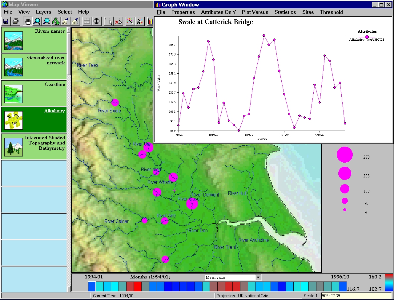
The LOIS Overview CD-ROM holds much diverse environmental data and model results. LOIS ran for six years (1992-1998) and involved some 250 scientists, producing an immense amount of multidisciplinary data of various types and formats. There are some 39 different types of data, or features, which include river, marine, and intertidal monitoring sites, river catchment, marine ecosystem and sea-level change model results, boreholes, and remotely sensed images. Additionally, it features ancillary data such as place names and a land cover map. To complement these, approximately 450 attributes have been measured at these feature types such as metals, nutrients, microcontaminants, invertebrates, foraminfera, ostracoda, and other physico-chemical determinands. Much of these data vary through time as can be seen in Figs. 1 and 2.
Fig. 1 Time series plot of alkalinity at a river monitoring station.
The range of temporal scales implicit in the data is large – every 15 seconds in the case of marine cruises, through to 1000 year intervals for a sea-level change simulation beginning in the Holocene period. Similarly, depth measurements range from millimetre accuracy in boreholes through to 1800m depths at the continental shelf edge, while planimetric scales range from intertidal monitoring sites covering a single beach, to hydrodynamic model output spanning the British Isles and North Sea.
Now that the scene has been set in terms of challenges and data, the system development and results of that development will be described in more detail.
Environmental information systems have advanced significantly during the past decade. Improvements in computing technology and contemporary development tools such as Microsoft Visual Basic, combined with object libraries and controls have provided developers with a powerful suite of tools for building flexible information systems. Today, scientific users demand a high standard of software product whether they are developed by large software houses or smaller bespoke developers. They require simple to use, clear and well presented geographical interfaces, powerful query and search capabilities and access to a myriad of datasets. Attempting to meet these requirements, and to some extent demonstrating to the user community what can actually be achieved, has been the responsibility of a small development team based at Plymouth Marine Laboratory (PML) and the Institute of Hydrology (IH).
Traditionally, software development projects within NERC have been undertaken in isolation. Many of these projects, however, share three essential components: mapping/data visualization, data storage/retrieval and data loading. Developing such software independently causes duplication of effort resulting in higher development and maintenance costs (Pressman 1994). The need to produce an integrated system for the LOIS programme and the problems associated with uncoordinated software development between projects, provided a good opportunity to revise our software development plan. It was identified that the majority of our software products would benefit from a generic modular development strategy. Large, monolithic software products that have not been developed in a well-designed modular way usually lead to systems that are extremely complex and often become nearly impossible to understand (Pressman 1994). Each of the essential components, mapping and data visualization, data storage and retrieval and data loading should be designed and implemented as discrete parts.
To understand and model the environment, large volumes of diverse data are required that vary in both space and time. These data must be effectively stored and managed so that relationships between datasets can be explored. In order to achieve this it has been the aim of the development team to design and implement a generic data model called the Water Information System (WIS). The name WIS in the context of STEM is somewhat misleading because of its direct association with water. WIS is a generic data model capable of holding many types of data even if they are not environmentally related. WIS only retains this name for historical reasons.
One of the key drivers behind the WIS data model has been the need to store numerous data types that vary in both space and time. WIS is a generic data model that can be implemented in virtually any relational database management system (RDBMS) (Moore 1997). Before detailing the WIS data model, it is worth considering the current approaches to the storage and organization of both spatial and temporal information with regard to current GIS products.
So far, the efforts of the mainstream database vendors have done little to impact the progress of GIS implementation. Traditionally, spatial data has been considered different in some respect to other corporate data (Newell 1997). During the past decade, it has become clear that spatial data is no different from any other corporate data. Spatial data may vary in time, require integrity checks, multi-user access, security and backup procedures. It is still unclear where the responsibility lies for data management issues as discussed above. Are they the responsibility of the GIS vendors or the DBMS vendors? It is the belief of the development team that both spatial and temporal data should be stored together in a unified database system (Moore 1997). This design philosophy and overall objective is also supported by (Peuquet and Qian 1997) who suggest "Our goal is to integrate all spatial, temporal and feature dimensions of geographic data in a unified and mutually supporting fashion. Such a dimensional integration not only makes all dimensions of the data accessible to the user, it also enables the user to observe and analyze from varying dimensional perspectives within a single representation."
As discussed by Batty (1992), GISs tend to store their data in one of two ways: in proprietary or hybrid formats.
Proprietary formats are developed by GIS vendors who wish to store their geographical data in specialized data structures. Specialized data structures often have performance advantages over equivalent database storage options. However, proprietary formats do suffer disadvantages in terms of flexibility and ease of integration with other software products and can be problematic in terms of data management issues such as multi-user access, integrity, security and backup procedures.
A hybrid approach stores geographical data in specialized data structures and attribute information in a DBMS. This approach offers the benefits associated with proprietary systems but also improves the data management issues associated with attribute data. The hybrid approach is still a compromised solution and causes some difficulties in terms of data integrity, security and application integration.
Neither of the above approaches was suitable for the STEM requirements. Therefore, the WIS data model was adopted. The WIS data models primary objective is to enable any object or feature to be recorded as it moves through space and time. Many of the current GISs are unable to do this effectively. A reason for this is suggested by (Peuquet and Qian 1997) "Current data representation techniques for Geographical Information Systems (GIS) are geared towards representation of static situations. Cartography has traditionally focused on the visual presentation of a proportion of the world at a specific point in time."
The WIS database design is best described in two parts, firstly the logical database design and secondly the physical database design.
The logical database design provides a simple conceptual model that helps users and developers to visualize how their data are stored. It allows the user to record the history of any object, or feature as it moves through space and time (Moore 1997). Descriptions of features and the events observed at them are recorded in terms of properties or attributes. Thus, to store river water quality data, an individual monitoring site might be classified as a feature and the variables which describe or are observed at the site, such as its position, the site name, a unique reference number, river flow, pH values and so on, would be its attributes. Other examples of features could include a river network, land use map, and satellite images. The terms feature and object/attribute and property are synonymous for the purpose of this paper. WIS supports a wide range of spatial and non-spatial data types allowing the user to record most types of variables. Both features and attributes are decided and defined by the users and their system and user definitions are stored in data dictionaries.
One of the significant advantages of the WIS data model is that all attributes or properties are assumed to be potentially time variant. Even positional properties may form a time series. For example, although a land based river monitoring station has a grid reference that is unlikely to change, marine and airborne sampling campaigns are conducted from a base that is constantly moving.
Unlike many GIS systems, the WIS data model does not have a predefined concept of a map or thematic layer. WIS stores objects, properties, and relationships as discrete entities. A map layer is a function of mapping/visualization software. For example, a map layer could contain several different features or object types.
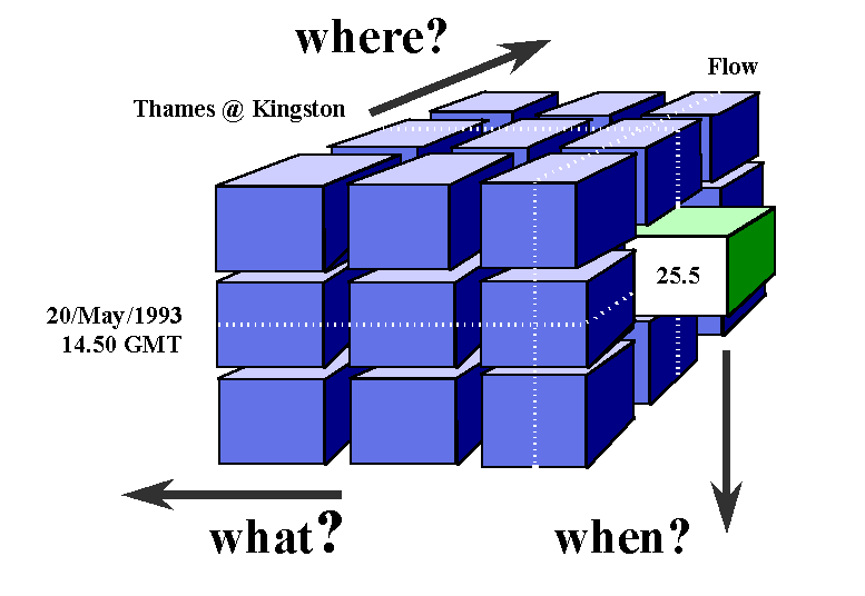
The text above describes the conceptual view of the data model. Fig. 3 provides a pictorial view of the WIS logical data model. The model holds data in a cube that is comprised of individual cells.
Fig. 3. The WIS logical data model. The WIS cube.
The three axes of the cube represent features (where observations are made), attributes (what has been observed) and time (when the observations are made). Each cell contains a value (or values depending on the attribute’s data type) of an attribute describing a feature at some moment in time. For example, one cell might contain a real value representing the rate of flow in the river Thames at Kingston on the 20th May 1993. There are no constraints on the number of features, attributes or occasions that can be stored by the cube other than that imposed by the physical limits of the hardware. Listed below are the key properties of the WIS cube:
The significance of the cube is that it provides a completely generic data independent structure around which to build equally generic tools for data visualization, analysis, retrieval and data loading.
The WIS cube can be implemented in any RDBMS. The underlying tables contain three different types of data; data tables, list tables and reference data.
The data tables share a common basic design and vary only in that different data types need different columns to hold the values. Each row in a data table contains a value from a cell in the cube. The first three columns of a data table contain the cube co-ordinates of the value, for example every value will have a feature ID (FID), a determinand ID (DID) and time ID (TID). For simple data types a fourth column holds the value. Thus, the DT_REAL table contains real values stored in a column called RVAL. However, more complicated data types such as points are stored in the DT_POINT table and require three columns called X, Y and Z to represent their values. Other data types include names, character data, line data, grid data and binary (OLE) objects.
The WIS search and select model relies on the concept of lists. A list contains a set of feature identifiers, attribute identifiers or date/time ranges that pick out the data required from the cube. For example, a ‘where’ list contains a set of features of interest. A ‘what’ list contains a list of attributes of interest and a ‘when’ list would contain a subset of the time axis. Combinations of what, where and when lists are also possible as in a ‘where/when’ list. An individual list is created by constructing the equivalent of a ‘where’ clause in a Structured Query Language (SQL) query. Complex queries are possible by using set operators on lists, such as UNION, MINUS and INTERSECTION.
Sophisticated facilities for time matching are a function of either the application software or the database interface. Many problems arise when values relate to different periods of time; some referring to an instant, others a day and yet others to a month or year. For example, a problem in the past has been that rainfall data are attached to rain gauges and river flow data are attached to gauging stations. Selecting flow data for occasions when it was raining was difficult on most systems. The problems associated with querying the time dimension of a 4D-GIS is easily the subject of another paper and will not be explored here.
Reference data provide supporting information such as units of measurement, periods, field and structure definitions, feature type definitions and attribute information.
It is our aim to ensure that users and to some extent developers are unaware of the physical implementation of the data model. Due to the data model’s generic nature, constructing queries in SQL for a novice user with only a limited understanding of the physical design could prove difficult. It is not recommended to access the data model directly via SQL as vital integrity and validation checks can be bypassed. In order to provide a conceptually simple and well-structured approach to data access a WIS database control was developed.
Application writers, programmers and modelers often want to interface directly with a WIS database at a low level. This method of access is achieved by the WIS database ActiveX control. The WIS control has two roles: to make access easy by providing a programming object model that specifically facilitates access to the WIS data model and to protect the database from corruption. The WIS ActiveX control has been developed for a product called Micro Low Flows (MLF). MLF is a PC based package that has been designed for the rapid estimation of low flow statistics from catchment characteristics at gauged and ungauged sites (NERC 1996). This product has been developed as a collaborative venture between IH and the UK’s Environment Agency and takes full advantage of the generic data model described in this paper. Encountering the same software development difficulties described earlier, the MLF development also decided to adopt and fund the future development of the generic data model.
The WIS control provides a structured object model that provides methods and properties that enable the user to select, update and maintain a WIS database. Querying a generic data model is always more difficult than a specific one. This problem is overcome by using the Get or Select methods that are provided by the control. Internally the control generates the SQL statements required to answer the programmer’s requests. Each method provides a flexible argument interface so that a variety of operations can be undertaken on the target database. The overall aim of the WIS control is to allow the programmer to conceptualise the data at a logical level whilst not concerning themselves with the complexity of the data models physical implementation. For example, a programmer does not need to know any of the table names or their relationships in the underlying WIS database to make full use of it.
Security, backup, concurrency, integrity, version control and auditing are some of the most important issues relating to data management. As discussed earlier both proprietary and hybrid data storage solutions for GIS do not meet many of these requirements. Storing both spatial and temporal data in one physical relational database automatically inherits all of the associated benefits that are typical of most RDBMS. As we develop systems that will be used by regulatory bodies it is important that issues relating to quality control and quality assurance are addressed. This process is only achievable if a holistic approach to data storage and management is adopted.
One initial important design decision was to develop a system that is freely distributable. Consequently many commercially available mapping systems could not be used. This, coupled with the lack of time and depth based systems meant that a completely new mapping package was required. The target audience for the CD-ROM ranged from schools and universities through to government agencies and industry. A second requirement, therefore, was that it was easy to use. The mapping component of STEM has been developed using a combination of Visual Basic, Windows API and OpenGL, which enabled the rapid development of a user-friendly graphical user interface.
Data are accessed via a query wizard that guides the user through the query procedure. At each stage SQL queries are made to the database to retrieve the relevant information for the user. After choosing a selection area on the map, the user may choose up to five feature types within a query. This means that the user may, for instance, retrieve chlorophyll data for a number of features, including river monitoring stations, marine monitoring stations, intertidal monitoring stations and so on. This is scientifically important when investigating the transfer of materials between different environments. The next stage in retrieving data is to select the attributes that are required. Again, a maximum of five may be selected, which is useful when comparing parameters, e.g. nitrate versus salinity. The user then specifies what time range is required.
When displaying data on a map that varies through time, it makes little sense to plot every value on the map at the same time. Later data may mask out earlier data and in a marine environment where the media will have moved in the intervening period the map will be misleading. A solution to this is to aggregate the data into periods of time (Kraak and MacEachren 1994). At present, STEM enables the user to aggregate in terms of years, quarters, months, weeks, days and hours. Similarly, it is necessary to aggregate the data in terms of depth, where present, to a user specified interval.
At the end of the query all attribute data throughout the time and depth ranges are retrieved into one map layer. Due to memory limitations the number of time periods is currently restricted to 200 time slices and depth grouping to 100 intervals. The data are aggregated into a statistical array associated with the map layer. Any time/depth combination may be chosen for display. This means that one STEM map layer may represent the equivalent of up to 100,000 (200 times x 100 depths x 5 attributes) of what might be described as conventional GIS map layers. Some depth/time queries may take several minutes within STEM, but when you consider how long it would take to create 100,000 layers in many current commercial applications, the advantages are clear.
There are several ways in which the time and depth dimensions are visualized within STEM. The main access to these dimensions is afforded through the time and depth bars that appear below the map window. The time bar (Fig. 4) represents each of the time periods selected in a query. Initially, the data displayed on the map shows the first period. The user may then select any of the segments in the time bar to change the display. The segments are coloured according to the mean value for all sites in that query. Hence, the time bar itself provides a useful summary of temporal variations in the dataset, e.g. seasonal variations in river quality data. Colours in the time bar and points displayed on the map may also represent other statistics, including measurement frequency, minimum, maximum and standard deviation. The depth bar behaves in a similar fashion and switching between the two dimensions is relatively seamless.
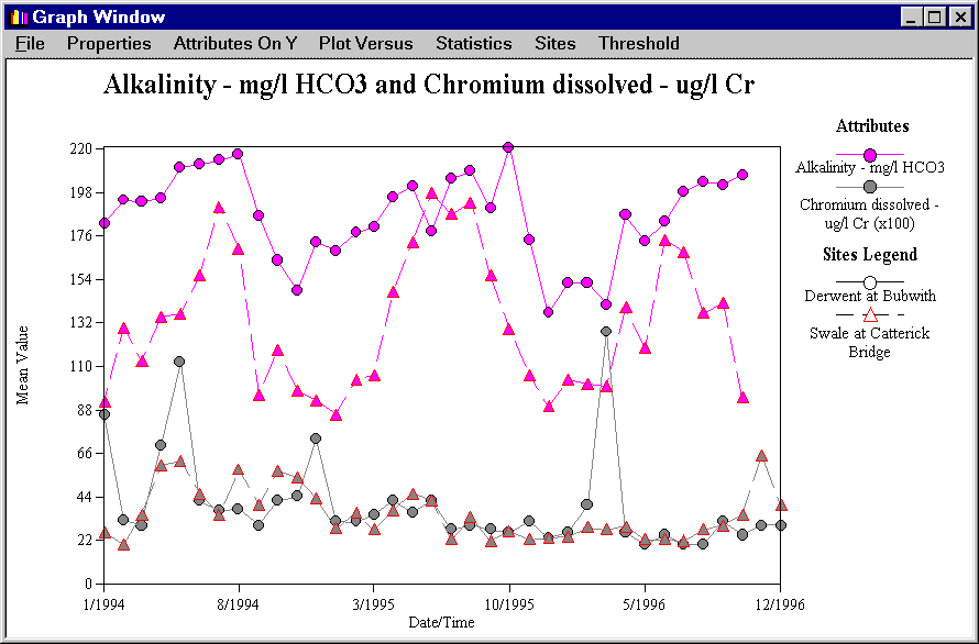
The second method is to produce time series or depth plots of the data. This is achieved by simply clicking on a site in the current map layer. Up to five sites and five attributes may again be compared within the graphing tool (Fig. 5). At this stage it is also possible to display the full time or depth series in addition to the calculated statistics.
Fig. 5. Graph showing a time series for alkalinity and chromium dissolved for two different sites.
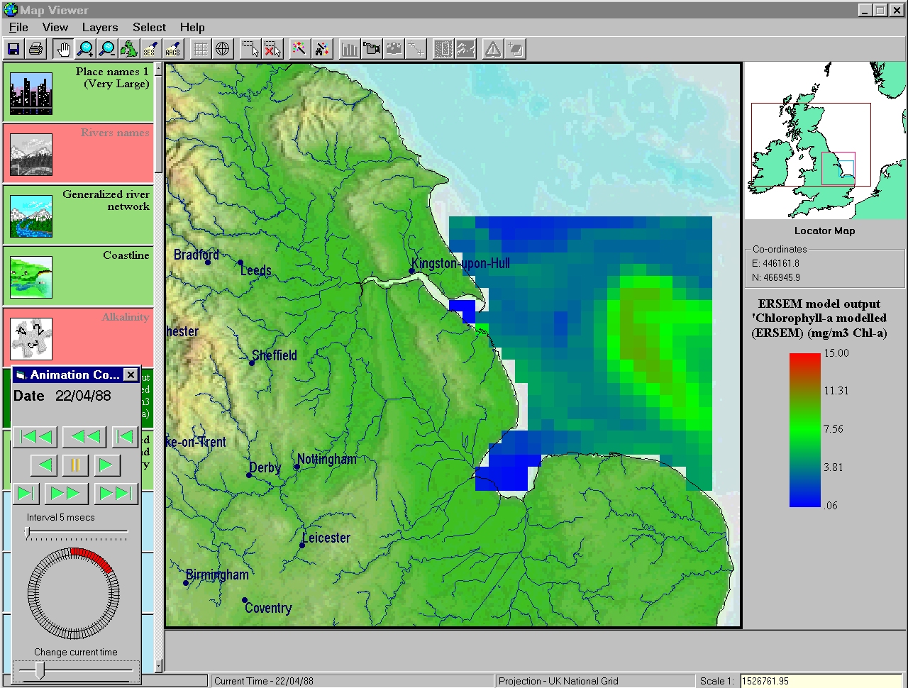
A further method, which applies to both point and raster data, is that of animation. An animation tool (Fig. 2) allows the user to control the speed, direction and extent of the animation. Animation of point data (e.g. concentrations of atrazine at fixed sites) may result in pulsating proportional symbols on the map or fixed-sized symbols that vary in colour during the animation. Alternatively, if more than one attribute has been retrieved it is possible to animate bar charts at each site, allowing a comparison of all parameters throughout the time sequence. Raster animations may include a set of remotely sensed images or the results of a model run.
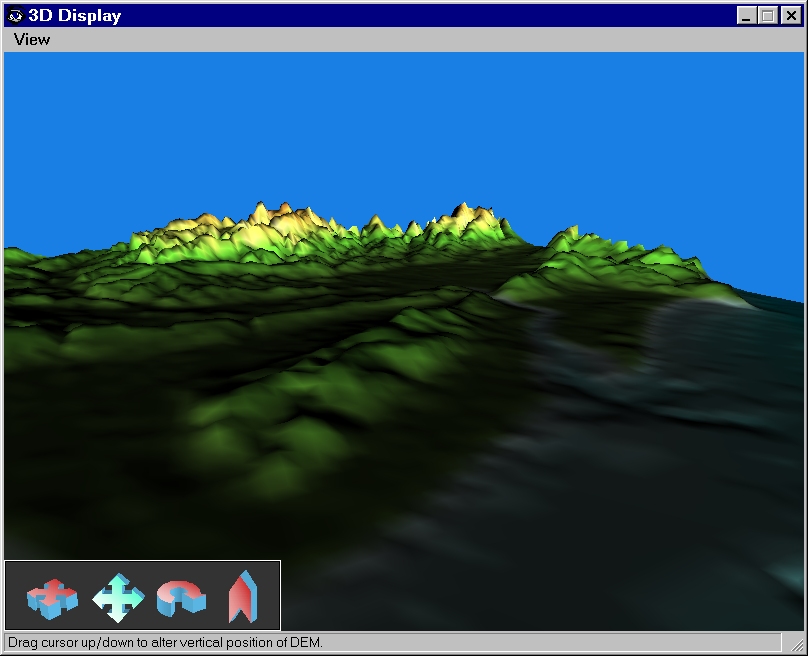
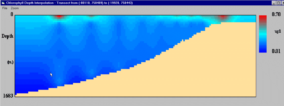
Depth is also visualized through depth profiles and perspective views (Fig. 6). Depth profiles are achieved by drawing a transect on the map and then performing an interpolation through depth (Fig. 7). It is hoped that the perspective view tool will soon be extended to incorporate all environmental data rather than simply an elevation surface.
Fig. 6. A perspective view of the East Coast of England, showing elevation and bathymetry.
Fig.7. An interpolation of chlorophyll profiles at the Hebridean shelf edge.
Many of the scientists involved in LOIS acquired data for their owns purposes, using their own instrumentation and possibly in different units, e.g., the marine scientists often measure using moles while the hydrologists use g/l. Some of the instruments used were intercalibrated, but unfortunately not all. All other identical attributes were converted to the same units.
Integration was also afforded by the development of an ‘integration wizard’. This differs from the query wizard in that the user initially selects an attribute rather than a feature type. The appropriate feature types to include within the query are determined behind the scenes. Within the query wizard the attributes are grouped into dictionaries (e.g. physical, chemical), while the integration wizard groups attributes into topical themes (e.g. nutrients, metals, microcontaminants, biology). This is more suited to the user who wishes to find an attribute in their field but does not necessarily know where (or at what feature) they have been measured. It is possible to include individual attributes in more than one topic and in the future STEM will enable the user to change the topics and dictionaries according to their own preferences.
The techniques, outlined in this section, provide some new tools for the scientist investigating their data. It is now very simple to compare attributes through time and across scientific disciplines, by graphing and animations. The benefits of this will hopefully become apparent as STEM is used in the scientific and academic communities.
The size of some of the databases used with STEM is continually growing. With this expansion, the need for guidance through the database will increase. Users will always ask fundamental questions of the data such as ‘What data exist?’; ‘How do I get them?’ (ESRI 1995). Presently, the databases are not too large for the user to answer those questions with simple exploration. However, there will come a time soon where the database is sufficiently large for such exploration to become an unrewarding and laborious process. Given this situation metadata issues will become important in future development.
The use of metadata can already be seen in STEM. The time and depth bars form a summary of the data (aggregated by average, measurement frequency etc.) at each period or interval, guiding the user to the most interesting datasets before seeing them in full. Alternatively, point data can be interrogated to give information about attributes measured there. Finally, the query interface (or ‘query wizard’) provides an overview by listing feature types, attributes at those features, and the time and depth ranges for those attributes.
Other future issues include:
The WIS data model now also forms the core of MLF and provides the flexibility to hold numerous data types in the future. The combination of powerful flow regime estimation facilities with generic mapping, data storage and data loading tools, opens up many opportunities for powerful water resource management tools.
The LOIS Overview CD-ROM has now been published and has demonstrated a GIS capability that incorporates time and depth. Environmental data can now be stored, accessed and visualized in a novel way that treats time and depth as valid dimensions within the system. We feel that STEM can now be used for all types of environmental data and indeed any other data which can be referenced in terms of time and space, e.g. crime/health statistics or house prices. As STEM is now used in the scientific community we hope that it will lead to discoveries about environmental data that were either not possible previously or took a long time to achieve.
The modular and generic nature makes the system suitable for expansion, including the addition of specialist scientific/analytical components and the progression into a fully functional corporate system. The system is already moving towards this goal and is being used by environmental institutes/companies in the United Kingdom.
We would like to thank Alex Les, Rob Patrick and Roger Moore who have helped, in no small way, to the development of the software and this paper. We are also grateful to the LOIS Data Committee, the LOIS Data Centres and everyone else involved in collating the data for the LOIS Overview CD-ROM.
Allen, J.I., 1997, A Modelling Study of Ecosystem Dynamics and Nutrient Cycling in the Humber Plume, UK, Journal of Sea Research, Vol. 38, Nos. 3-4, pp.333-359
Batty, P., 1992, Exploiting relational database technology in a GIS, Computers and Geosciences, Vol.4, pp.453-462
Ehlers, M., Beard, K., Haggerty, P. and Pearce, B., 1990, Synergistic integration of remote sensing, GIS/database technology and numerical modelling for marine geographic information systems, Remote Sensing Science for the Nineties, Vols 1-3, Ch.604, pp.949-952
Hill, D.R. and Bellamy, S.P., 1996, Search mechanisms for querying the time dimension in 4-D GIS, 1st Int. Conf. in Geocomputation, Leeds, U.K., University of Leeds, Vol. 1,pp.405-420.
Environmental Systems Research Institute (ESRI), 1995, Metadata Management in GIS, ESRI White Paper Series.
International Ocean Systems Design (IOSD), 1999, Fuzzy logic to manage coastal regions, International Ocean Systems Design, January/February 1999, pp.4-6.
Kemp, Z. and Kowalczyk, A., 1994, Incorporating the temporal dimension in a GIS, Towards temporality in GIS, Innovations in GIS, Warboys, M. (Ed.), Taylor and Francis, London, pp.89-103.
Kraak, M.J. and MacEachren, A.M. 1994, Visualization of the Temporal Component of Spatial Data, Advances in GIS Research: Volume 1 – Proceedings on the Sixth International Symposium on Spatial Data Handling, Waugh, T.C. and Healey, R.G. (eds.), Taylor and Francis, London, pp. 391-409.
Moore, A.B., Morris, K.P., Blackwell, G., Gibson, S.E. and Stebbing, A.R.D., 1999, An expert system for integrated coastal zone management in LOIS: A geomorphological case study, Marine Pollution Bulletin, In Press.
Moore, R.V., 1997, The logical and physical design of the Land-Ocean Interaction Study database, Science of the Total Environment, pp137-146.
NERC, 1994, Land-Ocean Interaction Study – Implementation Plan for a Community Research Project, Natural Environment Research Council, Swindon, U.K.
Newell, D., 1997, Perspectives in GIS database architecture, Advances in Spatial Databases, Vol.1262, p.377
Peuquet, D. and Qian, L.J., 1997, An integrated database design for temporal GIS, Advances in GIS Research II, 7th Int. Symp. On Spatial Data Handling, Delft, Taylor and Francis, Ch.68, pp.21-31.
Pfaltz, J.L. and French, J.C., 1994, Representing spatial change in environmental databases, Environmental Information Management and Analysis: Ecosystem to Global Scales, Michener, W.K. et al. (Eds.), Taylor and Francis, London, pp.127-138.
Pressman, R.S., 1994, Software engineering – a practitioner’s approach, McGraw-Hill, London.
Raper, J. and Livingstone, D., 1995, Development of a geomorphological spatial model using object-oriented design, International Journal of Geographical Information Systems, Vol.9, No.4, pp.359-383.
Stafford, S.G., Brunt, J.W. and Michener, W.K., 1994, Integration of scientific information management and environmental research, Environmental Information Management and Analysis: Ecosystem to Global Scales, Michener, W.K. et al. (Eds.), Taylor and Francis, London, pp.3-19.
Strebel, D.E., Meeson, B.W. and Nelson, A.K., 1994, Scientific information systems: A conceptual framework, Environmental Information Management and Analysis: Ecosystem to Global Scales, Michener, W.K. et al. (Eds.), Taylor and Francis, London, pp.59-85.
United Nations Environment Programme (UNEP), Guidelines for Integrated Management of Coastal and Marine Areas, (UNEP Regional Seas Reports and Studies, 1995), No. 161.
Wachowicz, M. and Healey, R.G., 1994, Towards temporality in GIS, Innovations in GIS, Warboys, M. (Ed.), Taylor and Francis, London, pp.105-115.