Return to GeoComputation 99 Index
David Martin and Fulong Wu
Department of Geography, University of Southampton, Southampton, SO17 1BJ United Kingdom
E-Mail: D.J.Martin@soton.ac.uk,
F.Wu@soton.ac.uk
This paper describes the application of CA to the simulation of urban growth in the south-east region of the UK, an area currently subject to considerable development pressure. The actual settlement pattern is initially modelled as a fine resolution grid using a population surface modelling technique originally developed for use with census area centroid data, (Bracken and Martin, 1995) but here applied to unit postcode information which offers greater spatial and temporal resolution than that available from the population census or conventional land use mapping. This application is a further development of SimLand (Wu, 1998a) which makes use of Arc/Info for spatial data management, with AML programs to permit the evaluation of a range of alternative local and regional constraints on the development process. We classify the wide variety of factors affecting development into static and dynamic ones. The success or failure of a seed becoming a developed land use depends on their combined effect on the self-organised process of local growth. This is further dependent upon the threshold which allows such a process to proceed. From the observation of land use states in two time periods, the distribution of land use changes is identified. In general, the threshold and its transformation are used to reflect three types of inputs: the growth rate which is related to economic activity, regional variation and policy control. With different thresholds applied, simulation can generate a series of scenarios of urban development. Development scenarios are treated not as place-specific predictions, but as possible realizations of the development process, from which a number of structural indicators can be derived. This research has a number of original features: it uses detailed empirical spatial data on a fine resolution grid; it integrates global effects with the local self-organisation mechanism of urban growth in a more explicit and parameterised way; it utilizes GIS functionality and thus provides a closer integration with other decision-making tasks; it searches the parameter space through a computationally intensive approach; and finally it uses structural indicators to compare the simulation results with the reality.
Simulations using CA have been widely applied. However, early attempts were typically more in the nature of metaphors of urban growth with little explicit relationship to underlying behaviour theory (Couclelis, 1985; Batty and Xie, 1994). It is now becoming clear that the CA approach is essentially heuristic and therefore attention should be drawn to the plausibility rather than the 'correctness' of models. With a better understanding of the technique, CA simulation is at the stage of exploring more complex behaviours. In the literature, a variety of ways of defining the transition rules of CA models have been reported (White and Engelen, 1993; Batty and Xie, 1994; Wu and Webster, 1998). These exercises highlight the need for an integrated approach which combines CA's relatively simple abstraction with the behaviourally richer models of urban processes found in the social sciences (Webster, et al., 1998). The obstacle to incorporating the richness of urban models is not due to technical difficulty but rather the theoretical justification for a complex model. The notion that CA reveals complex global patterns as they 'emerge' from a set of simple local transition rules is absolutely right but urban development, for example land use conversions, are unlikely governed by simple rules. This becomes increasingly apparent as shown in the studies of political economy of urban land uses. With all these CA approaches a critical question remains regarding the way the transition rules should be interpreted in economic or other behavioural terms. The behavioural aspect of most CA simulation is still weak.
Despite a variety of modelling approaches, we can envisage a two dimensional matrix to generalise a general framework (Figure 1). The two dimensions are global vs. local rules adopted and the empirical vs. theoretical configuration. At each extreme, there are some well-known models. The strictly local rule associated with a pure theoretical configuration is often used in simple metaphoric models. These models follow some well-defined physical processes such as diffusion-limited aggregation (DLA) to simulate generic urban forms. Fractal properties are often presented as they can be seen in real-world cities (Batty and Longley, 1994). The insights generated from these models are not directly applied in the control of urban growth because of the abstraction of the model but they are useful in the sense of analogy - the fundamental similarity between the morphology of theoretical and real cities suggests a similar process might in fact provide a plausible characterisation of urban growth. Lying at the other extreme are empirical and global models, which are often "operational" and based on GIS. These typical cartographic models use methods such as map overlay and buffering. Factors affecting urban development such as access to roads, distance from the city centre, topography, and land uses are presented as may layers and superimposed and manipulated to generate the final "suitability" index. Often such a process is applied to the whole map area. The method is essentially static. More sophisticated cartographic models can be formalised through map-algebra. At this extreme are also empirical population density models. These models are built up from disaggregated spatial units and calibrated through statistical methods. While they may provide insights into how the population density is related, in a regression sense, to a bundle of locational factors, they do not describe the processes of population density change because a simple extrapolation of existing relationships is problematic. As shown in recent studies on the dynamics of urban spatial structure, the population density surface is of emergence nature, in the sense that a monocentric structure can evolve into a polycentric one if the same relationship is applied repeatedly (Wu, 1998b). The theoretical foundation of conventional urban models, however, is neoclassical urban economics that assumes the urban systems are always at equilibrium. The well-known theoretical model based on this assumption is the Alonso (1964) urban land use model. Most models in this category are theoretical ones with limited connections to the practices of urban and regional planning. But the city is a self-organising system, as shown by the pioneering work of Peter Allen in the 1970s (Allen, 1997). Between these extremes there are a vast number of hybrid models that mix the global and local rules and use different spatial resolutions and hence different realism of urban configurations.
We believe that the design of an appropriate simulation strategy should consider the purpose of modelling and that the urban growth processes can be best articulated at a certain level of abstraction and balance of empirical vs. theoretical, global vs. local dimensions. In this research we propose a framework which allows such an appropriate simulation strategy to be implemented. We give explicit considerations to the parameterised global and local factors affecting urban growth.
In this work, we assess the development potentiality according to a number of key factors which will be discussed in detail below. Based on this assessment we use the Monte Carlo method to generate development seeds. This seeding process reflects the positive effect, i.e. stimulation of development factors on urban growth. As this is calculated globally, the emergence of seeds can be seen as the process used in conventional modelling but subject to stochastic effects. The multi- regional development factors, however, also play a constraint role. In this simulation, the constraint effect is only based on regional population growth projections. If simulated growth exceeds target growth, sites subject to development pressure will be randomly selected so as to fit the overall constrained rate of growth.
The seeding process reflects the spontaneous nature of urban growth but the history and existing land uses affect the development as well through local interactions. This is the self-organised aspect of urban growth. To reflect such a characteristic, the development situation is evaluated in a 3 x 3 local kernel, based on the development state at time t. This is a standard CA rule definition. The strength of local growth is calculated as the ratio of developed land to undeveloped sites but in the second model we introduce a more sophisticated measure to reflect the combined global and local effects. The local development pressure is then compared with a threshold to decide whether the site in question can be chosen as a potential development site. The threshold is a critical parameter which reflects how self-organisation might be started. An initial value is used but it is then adjusted according to the projected rate of growth. If the potential growth is lower than the projected one, the threshold will be lowered which means that it is easier for a self-organised process to start off. This adjustment is made during the simulation in which the threshold value varies from iteration to iteration. In theory, the threshold adjustment can reflect three types of effects: the growth rate which is related to population and economic activities, regional variations, and policy control. As a general framework, more rules can be defined separately for failed sites and successful sites but in this simulation we do not consider them to be controlled independently.
It is worth noting that the development factors in this simulation are updated according to the changed land uses at time t. In particular for the second model which will be elaborated later, development factors such as the local attractiveness are measured according to a gravity type of equation. The size of city clusters changes during the simulation and so does the distance to the nearest edge of settlement.
This method depends on the presence of centroid points for each small area for which population counts are available, and which may be considered to be 'population-weighted'. In the UK Census context, population-weighted centroids are provided by the census offices for each enumeration district (ED), the smallest zone used for the publication of census data in recent censuses. The surface construction algorithm visits each centroid in turn and examines its distance from other local centroids. This distance can be used as an indication of ED size in that region, and a distance decay function is calibrated and used to redistribute the population total at the centroid into the surrounding cells of a raster output matrix. Thus in areas of high population density, with centroids located close together, population may be spread very short distances from the centroid, reflecting small ED sizes. In remote rural areas, population may be spread over larger distances up to a predetermined maximum which is a parameter of the model. Thus many cells which in urban areas may recieve population from several different centroids, while others which are remote from any centroid remain unpopulated. The resulting model embodies a representation of the settlement geography which is one of its most important advantages over zone-based representations, and it is for this reason that we have chosen to use this approach to construct the initial model from which to run our urban development simulations. Although total population has been used in this example, the model may be applied to any count data present at the zone centroid locations. Other applications of census-based surface models produced using this approach, and again taking advantage of the reconstruction of the settlement pattern, may be found in Brainard et al. (1997), Lovett et al. (1997) and Mesev et al. (1995).
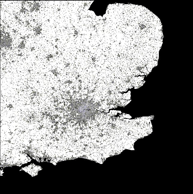
As the postcode geography has changed, the directory has been kept up to date and periodic revisions published which relate 1991 census EDs to contemporary postcode geography. No postcodes are removed from the file, but terminated and reused codes are flagged. New codes are assigned a grid reference and may hence be associated with an ED. The 1995 and 1997 versions of the file also contain a large or small user indicator for each postcode. Large user postcodes typically receive over 25 items of mail per day and are usually commercial addresses. Only the current postcodes have been used from each directory, allowing the resulting models to approximate to postal geography in 1995 and 1997. A household count of 15 has been assigned to any new small user postcodes for which household counts are unavailable, representing the typical number of addresses per household. There are thus around 850,000 data points available for surface modelling. These locations have been used to provide the centroids for the construction of surface models for a 300km x 300km area of the South-East of England, centred on the London metropolitan area, with a cell size of 200m, resulting in models with 1500 x 1500 cells. Household counts have been used as the variable for redistribution, so that each output model is effectively a household density surface. The basic household surface for 1997 is shown in Figure 2, in which unpopulated regions are shown as white, and increasing population density is represented by darker shades of grey.
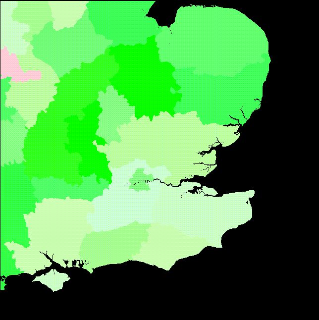
In order to constrain the amount of population growth occurring in the simulation models, a series of official population estimates based on 1993 mid-year population estimates at county level have been used. Overall, the area is due to experience around an 8% growth in population to 2016, with the largest growth in a band running from East Anglia, to the north east of the area, around the outside of the metropolitan area to Berkshire in the west. The major urban areas experience static population totals or a small decline. The study area covers all or part of 30 counties, for which population projections to 1996, 2001, 2006, 2011 and 2016 are available. A county map has therefore been created with associated growth rates to constrain the simulation within the officially projected population growth levels. A map of projected population change by county is shown in Figure 2. White represents no projected chage, with increasing green intensity representing projected growth, and red intensity projected fall in population.
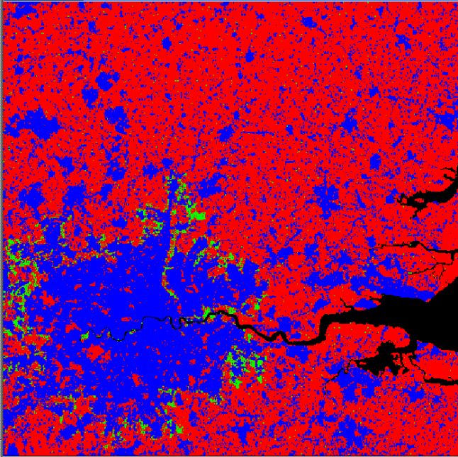
Major factors affecting the attractiveness of residential areas throughout the region include commuter travel times to London, and accessibility to the national motorway network. Commuters travel to London from everywhere within the study region, and the dominant mode of transport for this long-distance commuting is by train. A London travel time surface has therefore been devised by taking fastest travel times to the appropriate London terminus arriving between 0800 and 0900 on a weekday, as this represents the timing most likely to be used by commuters. Times have been obtained from 130 major stations. Commuter route information was extracted from McGhie (1992) and times were obtained from the Railtrack travel enquiry site at http://www.railtrack.co.uk/travel/. Travel times for each individual cell have been calculated by estimating travel time to the nearest station by crow-fly distance assuming a mean travel speed of 60 km/h, and these times have been added to the fastest available train time. Special treatment has been given to the Isle of Wight, in the centre of the South Coast, which is the only genuine Island in the study area containing a significant population, and for which travel times have been increased by an amount equivalent to the necessary passenger ferry crossings. In deriving the full travel time surface, the assumption has been adopted that if a major station is located within 10 minutes' drive time of a given cell, the commuter journey will be routed via that station. At greater distances, the shortest travel time to London is applied, regardless of the distance to the station which must be used. These general assumptions are felt to better reflect commuter behaviour than a simple Euclidean allocation of cells to stations. The travel time surface is illustrated in Figure 3, with increasing red intensity indicating travel time proximity to a London rail terminus, and regional stations shown as green point symbols.

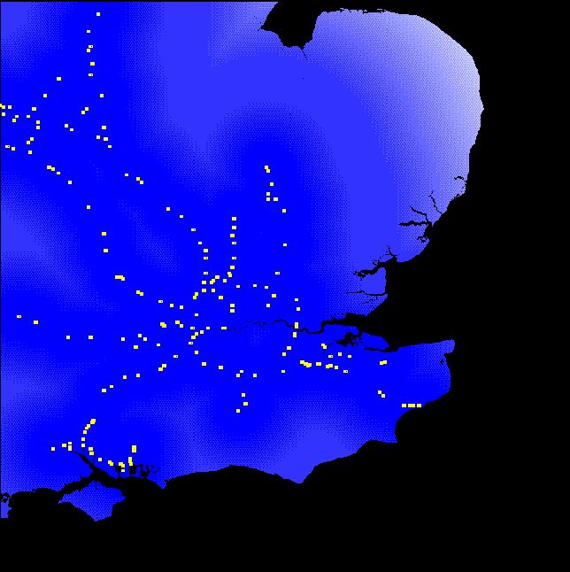
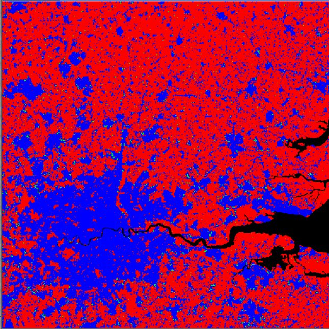
A further aspect affecting development potential in this region is accessibility to the national motorway network, and a complete set of motorway access points has been digitized, and distances derived to each cell. Only sections of motorway which are connected to the principal motorway network are included (thus no account is taken of short isolated lengths of urban motorway). The motorway access surface is shown as Figure 4, with increasing blue intensity indicating proximity to a motorway junction, and junctions shown as yellow point symbols.
The initial state of the land use is derived from the processed 1997 postcode coverage. We aggregated the large user postcodes, typically commercial users, with the small user postcodes, suggesting the boundaries of existing urban built-up areas. The surface has been constructed using custom Fortran programs, and contains estimated household counts in each cell, derived from the directory of enumeration districts and postcodes. This image provides the initial land use map on which we base our simulation. We assume that the expansion of urban built-up area is at the same rate of projected population growth, which is an 8% growth over the South-east region. In the model, however, we use the projected growth rates on the basis of counties. The target growth rates are then translated into the increase of the number of cells per iteration. The number of cells for new developments is then used as the constraint. The simulations are run over 23 years, which gives a final scenario of year 2020. The area that is not suitable for urban development such as sea and coastal water areas are coded as nodata and thus excluded from the site selection process.
The two major factors affecting the attractiveness of residential areas throughout the region are commuter travel times to London and accessibility to the national motorway network. The two surfaces are standardised according to the maximum and minimum values. Here we use a dynamic version, that is, we flag potential development sites on each iteration and then standardise these cells. Therefore, the attributes of these two factors always range from 0 to 1. These two attributes are then added to give the overall attractiveness for residential use. This can be seen as a standard land evaluation process in the form of the multicriteria evaluation (MCE). Basically, an evaluation score can be calculated by weighted summation of standardised development factors. But here we just use equal weights of these two development factors. This suitability score, however, is seen as a measurement of global attractiveness. The development of a site is further dependent on the local evaluation.
We use the Arc/Info GIS as a data management tool, together with AML programs to permit the evaluation of a range of alternative local and regional constraints on the development processes. The simulation model is a development of the SimLand (Wu, 1998a), but differs in that it treats the global and local evaluation in a more explicit way. In SimLand previously developed, the local evaluation is considered just as one development factor in the weighted summation of the suitability score. In this model, however, we treat the effect of local growth as a critical factor that finally decides whether the land use can be successfully converted. The general procedure is outlined in Figure 6. The strength of local evaluation is compared with a threshold to determine whether the self-organisation process can start off. The score calculated from the global development factors only determines the probability of seeding new development sites.
The seeding probability is based on the summation of commuter times to London and the distance to motorway junctions. However, it is obvious that the relationship between the score and probability should be non-linear in a similar form of logistic or Poisson distribution. Here, the site generating the highest score at the time of development is thought as a benchmark. The probability of this highest score site being developed is 1. The probability of development decreases with decreasing scores. The non-linear transformation is then used to depress the probability away from the maximum score in order to achieve greater discrimination between cells in any one simulation. In fact, this can be thought as some sort of distance decay - the probability of development decays along with the distance to the ideal site. The equation used is therefore:
 [1]
[1]
where ptij is the probability of land conversion from vacant to urban use at the location ij at time t; Rtij is the land suitability score at the same location at time t; Rtmax is the maximum score of land suitability at the simulation time t of calculation; and alpha is the dispersion parameter. The value of the dispersion parameter governs the stringency of site selection, with a higher value reflecting a more stringent selection process. We have tested the value in the previous simulation and thus in this model the value is chosen as 5.0.
The seeding sites are then generated according to the Monte Carlo process in which the probability score is compared with a random value. To control the seeding rate, not all sites will be considered. Instead, a fraction of developable sites are chosen. The ratio of this fraction to the total developable sites is another parameter which can be controlled in simulation, thus varying the model from a sort of CA to a conventional model. The sites generated from the seeding process, albeit non-deterministic, follow general global factors.
In this simulation, we consider the open space within the existing built-up area to be a special type of use, for example, cemeteries, parks and other protected urban spaces. These areas surrounded by existing development in the city area are frequently subject to planning controls and are therefore unlikely to be developed. We use a GRID function called "fill", often used in hydrological modelling to fill the sink of a surface, thus identifying these areas and preserving them during the simulation. Thus, although these areas are very attractive according to the multicriteria evaluation function discussed above, they are excluded from the consideration of further development. Two different approaches of computing local growth strength have been evaluated. The first model simply counts the number of developed sites in a 3x3 neighbourhood. The second model incorporates a spatial interaction equation to calculate the local attractiveness. This considers the size of each continuously extended settlement and the shortest distance to the edge of that settlement. To reflect a non-linear relationship, we use the logarithm of the size of settlements. The two methods will both lead to an attribute describing the strength of local growth. The value is then standardised on these sites available for development. The distribution of the score, however, is not controllable at each iteration because the attribute is calculated on the basis of a local kernel. The value further depends on the distribution of developed sites or the shape of settlements which differs from iteration to iteration.
The initial threshold adopted is 0.8 which means that sites seeing a local growth strength exceeding 80% of the strongest sites can be developed. This is then used to generate a temporary land use grid. The distribution of land development is then evaluated and the number of converted cells is summed over counties. For the counties in which the actual growth is lowered than expected, a lower threshold value is adopted to generate the final land use; but for the counties in which the actual growth exceeds the projected growth, these sites will be randomly selected. This is a simplified method of constraining the development rate to the target one, in consideration of the computation involved. Ideally, we can use a loop to adjust the threshold in small steps until it generates the target growth rate. The concept lying behind this adjustment of the threshold is that the process of self-organised growth is dependent upon the demand for land. When the demand is very high, in the sense that there is a gap between the supply from the existing method of development and the demand due to population growth, a slight growth might lead to more growth in the neighbourhood and finally much stronger agglomeration
The two methods, representing how development should agglomerate, may lead to quite different spatial forms. For a simple count of the local number of developed sites, a seed can lead to a more dispersed growth, because the seed is considered as equally important as the existing urban land plot. In the second model, however, the local attractiveness considers further the location of developed sites and the size of settlements. Thus, the area nearby a larger settlement is more attractive than the one locating nearby a small settlement or a scattered seed.
The initial 300 x 300 cell land use model derived from 1997 postcode information has 1.4 million cells which are excluded as sea. Of these, 297827 have urban land uses, spread across 37815 separate settlements (where a settlement is defined as one or more adjacent urban cells surrounded by undeveloped cells). In simulation 1, 12570 new cells are developed, compared to 10265 cells in simulation 2. This difference is accounted for by the use of county-level population projections to constrain the amount of development which is allowed to take place. The second model does not provide sufficient highly attractive cells for development to meet the population requirements of every county, and counties not adjacent to major urban areas remain underpopulated at the end of the simulation.
The two simulations represent rather different development constraints, resulting in alternative development patterns. Our primary concern in this paper is with an implementation of the proposed methodology, rather than with substantive urban development issues, but a brief exploratory analysis is given here, with some further comments on the ways in which the GIS environment could be used to interrogate the results. These models are not intended to predict whether or not development will take place at a particular site, but rather to provide a means of understanding the general nature of the development pattern which would result from a particular combination of constraints. Some initial approaches to the description of change between population surfaces is presented for the same region using 1981 and 1991 census data in Martin (1996b), and similar tools are used here.
Table 1 shows the distribution of the sizes of developments. The table shows for both simulations, the frequencies of settlements of different sizes (mesured by numbers of 200m x 200m cells). The continuously built up area of London comprises 36976 cells in the initial population model. In simulation 2, this area grows to a final size of 46934 cells, compared to 41005 cells in simulation 1. Similarly, the other largest urban areas grow to larger final sizes in simulation 2. It is important to note that the total number of cells developed is not the same between the two models, due to the working of the county-level constraints. It is not possible to provide direct measures of the population sizes of settlements changing at different rates, as the development process involves a high degree of merger of adjacent small settlements, and the absorbtion of small settlements into nearby large ones. Cross-tabulation with population estimates or a neighbourhood classification scheme would permit a more detailed analysis of the types of places most affected by new development under any given scenario.
| Number of additional cells | Simulation 1 | Simulation 2 |
| 1-3 | 25613 | 27496 |
| 4-15 | 10274 | 9645 |
| 16-63 | 1552 | 1612 |
| 64-255 | 274 | 309 |
| 256-1023 | 81 | 82 |
| 1024-4095 | 19 | 22 |
| over 4096 | 2 | 2 |
| Distance band (km) | Developed cells at start | Simulation 1 (%) | Simulation 2 (%) |
| 0-25 | 34250 | 1.5 | 6.3 |
| 25-50 | 45924 | 6.4 | 8.6 |
| 50-75 | 49150 | 5.4 | 2.3 |
| 75-100 | 46857 | 4.8 | 2.2 |
| 100-125 | 38281 | 4.6 | 2.1 |
| 125-150 | 36258 | 3.5 | 1.5 |
| 150-175 | 34223 | 2.8 | 1.3 |
| 175-200 | 13625 | 3.5 | 1.6 |
The objective of these simulations has not been to provide a single predictive model of urban development in the SE region of England to the year 2020. Rather, our interest has been in exploring the ability of CA simulation to produce plausible development scenarios in a real world situation, and to incorporate a range of both theoretical and empirical development constraints. We suggest that there is a valuable role for CA simulation in presenting alternative scenarios for future urban growth, which are based on detailed real-world data and constraints. This represents a combination of theoretical and empirical considerations.
This kind of application of simulation to real world scenarios must be linked to GIS in order to maintain spatial details and to take advantage of easy graphical manipulation and display. It would be quite difficult if not impossible to build the whole process of simulation outside GIS. For example, the special treatment of open spaces within existing urban areas makes use of a hydrologic surface function which is readily available in the GIS environment. Our exploratory analysis, which relates the resulting urban growth patterns to settlement sizes and distances from the urban centre are also dependent on the spatial functionality avialable within the grid modelling module of the GIS software. These examples illustrate how the available GIS functions can be readily accessed during simulation to avoid the need for reprogramming of spatial analysis functions. Considering the computational efficiency, a hybrid system that combines the GIS functionality and dynamic process models seems to be an appropriate solution.
Alonso, W. (1964) Location and land use. Harvard University Press: Cambridge, Mass.
Batty, M. (1998) Urban evolution on the desktop: simulation with the use of extended cellular automata Environment and Planning A 30, 1943-1967
Batty, M., Couclelis, H. and Eichen, M. (1997) Urban systems as cellular automata, Environment and Planning B 24 159-164
Batty, M. and Longley P. A., (1994) Fractal Cities. Academic Press, London.
Batty, M. and Xie, Y. (1994) From cells to cities Environment and Planning B 21 531-548
Bracken, I. and Martin, D. (1995) Linkage of the 1981 and 1991 UK Censuses using surface modelling concepts Environment and Planning A 27, 379-390
Brainard, J. S., Lovett, A. A. and Bateman, I. J. (1997) Using isochrone surfaces in travel-cost models Journal of Transport Geography 5 (2), 117-126
Couclelis, H. (1985) Cellular worlds: a framework for modelling micro-macro dynamics Environment and Planning A 17 585-596
Hägerstrand, T. (1965) A Monte Carlo approach to diffusion Archive of European Sociological, VI, 43-67.
McGhie, C (1992) The Royal Insurance London Commuter Guide Whitley, Good Books
Lovett, A. A., Parfitt, J. P. and Brainard, J. S. (1997) Using GIS in risk analysis: a case study of hazardous waste transport Risk Analysis 17 (5), 625-633
Martin, D. (1989) Mapping population data from zone centroid locations Transactions of the Institute of British Geographers NS, 14, 90-97
Martin, D. (1996a) An assessment of surface and zonal models of population International Journal of Geographical Information Systems 10, 973-989
Martin, D. (1996b) Depicting changing distributions through surface estimation in Longley, P. and Batty, M. (eds.) Spatial analysis: modelling in a GIS environment Cambridge, GeoInformation International 105-122
Mesev, V., Longley, P., Batty, M. and Xie, Y. (1995) Morphology from imagery - detecting and measuring the density of urban land-use Environment and Planning A 27 (5), 759-780
OPCS (1995) 1993-based subnational population projections PP3 No. 9, London, OPCS
Tobler, W. R. (1979) Smooth pycnophylactic interpolation for geographical regions Journal of the American Statistical Association 74, 519-530
Webster, C. J., Wu, F. and Zhou, S. (1998) An object-based simulation model for interactive visualisation Proceedings of the 3rd International Conference on Geocomputation, University of Bristol, 17-19 September 1998. http://www.ggy.bris.ac.uk/geocomp/cdrom/32/gc_32.htm
White, R. and Engelen, G. (1993) Cellular automata and fractal urban form: a cellular modelling approach to the evolution of urban land-use patterns Environment and Planning A 25 1175-1189
Wu, F. (1998a) SimLand: a prototype to simulate land conversion through the integrated GIS and CA with AHP-derived transition rules International Journal of Geographical Information Science 12, 63-82
Wu, F. (1998b) An experiment on generic polycentricity of urban growth in a cellular automatic city Environment and Planning B 731-752
Wu, F. and Webster, C. J. (1998) Simulation of land development through the integration of cellular automata and multi-criteria evaluation Environment and Planning B 25, 103-126.