Return to GeoComputation 99 Index

Dataspaces as an organisational concept for the neural classification of geographic datasets

Abstract

This paper describes some early experiments involving the use of the Self-Organising Map (SOM), and Learning Vector Quantisation (LVQ) algorithms--forms of neural-based pattern classifiers. A description is given of a combined classifier that can employ both supervised and unsupervised learning. Experiments using the SOM/LVQ to classify landcover at the floristic level show that with a careful configuration, the classifier is able to achieve good performance on a complex geographical problem. Further experiments are then conducted into a divide-and-conquer style of classification, using the traditional notion of a geographically-relevant dataspace to provide a hierarchical structure to the classification tool. Results show that the approach based on dataspaces leads to similar levels of performance, provided that the individual dataspaces are finely clustered using an unsupervised approach initially with supervised classification used to unite the separate dataspaces.

1. Introduction

Traditional geography and environmental analysis has often made use of the idea of a dataspace in order to add structure to the understanding of complex natural systems. A dataspace is some subset of the overall attribute or feature space where a specific geographical theme is represented. Examples are spectral space (say from remotely sensed data), geographic space (location and height), and environmental space (for example rainfall, soil pH, and barometric pressure). Data spaces offer the advantage of decomposing what is effectively a highly multivariate problem that may span several scientific disciplines into a number of coherent units where some common theme is represented.

It has been suggested that the relationships within these spaces are not the same as those between them (Aspinall and Lees, 1994), due to the inherently different structure of each separate domain. For example, a spectral dataspace may contain ratio data with a distribution that can be approximated by a Gaussian curve, whereas a geographic space may show strong clustering and directional trends that would need to be modelled in a different manner. To be useful for classification, a dataspace should contain strong internal cohesion so that the distribution of data might be modelled using simple and consistent metrics. Figure 1 shows four dataspaces representing different aspects of the complex environmental dataset used in these experiments.

The trend among statistical classifiers (such as maximum likelihood) and inductive learning techniques (such as decision trees and neural networks) is to treat the entire feature space as comprising a single descriptive vector. In geographic terms this is equivalent to the construction of an all-inclusive or universal dataspace. While this approach has met with success (e.g., Benediktsson, et al., 1990; Hepner et al., 1990; Civco, 1993; Fitzgerald and Lees, 1994; Paola and Schowengerdt, 1995; Freidl and Brodley, 1997), it seems likely that the mixing of concepts has a distinct disadvantage--the classification tool has effectively to 'learn' to disentangle data used in training. While strong clustering may exist within parts of the total space, it may be confounded by the 'noise' of unrelated (or weakly related) concepts. This would obviously complicate the learning task, which in turn may reduce classification accuracy. The counter argument to this is that each dimension may be useful for some discrimination task or other; furthermore, some tasks may require most or all of the dimensions in the data concurrently. The overall aim of this paper is to test the following hypothesis: That classification based on dataspaces can outperform approaches using the entire feature space in terms of accuracy.

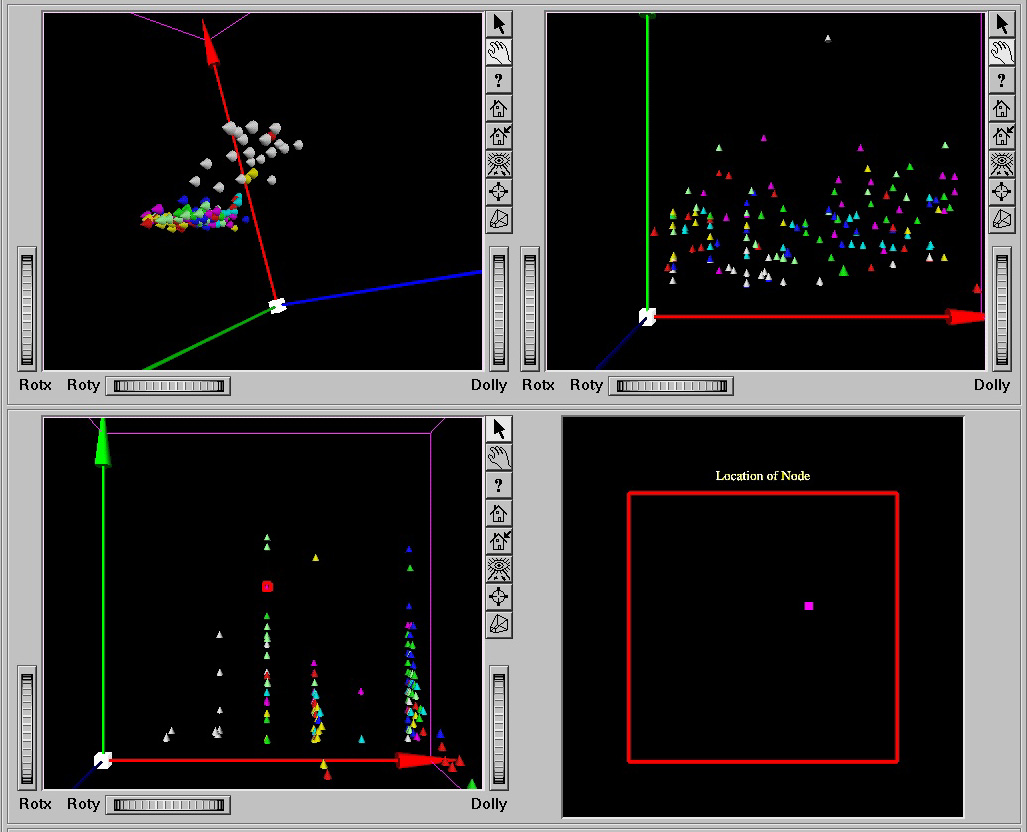
Figure 1. Four different dataspaces: Top left, spectral data from remote sensing; top right, landscape structure; bottom left, geology and hydrology; and bottom right, geographic (locational). Differences in structure between these spaces are clearly evident.

An obvious advantage of a 'divide and conquer' approach is that a different type of metric or model can be applied in each feature sub-space, according to its specific structure. Following a local process of classification or clustering within each space, a new space of part-classified dataspaces can be produced and then mapped via a final classification stage to the target output classes. Figure 2 shows the architectural arrangement of both a combined and a partitioned feature space.

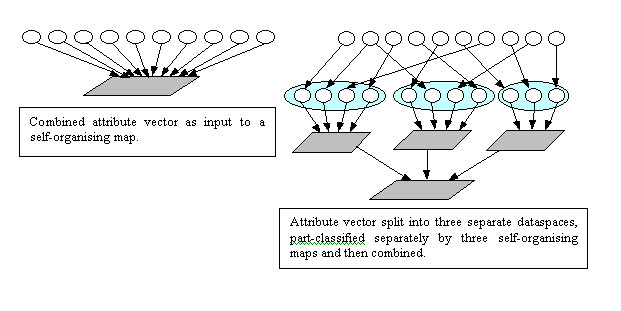
Figure 2: A comparison between typical approach to classification, and the structured hierarchical approach taken by a Self-Organising Map (SOM) based on attributes grouped into dataspaces.

There is, in principle, nothing to prevent each dataspace being handled by a completely different type of tool, leading perhaps to ensembles of classifiers (Dietterich, 1997); however, for simplicity, here we adopt a consistent neural technique for each space. Of the many different types of neural networks that have been proposed (see Bishop, 1995 for a useful overview), several might be considered viable. For example, a modified feed-forward backpropagation network (Gahegan et al., 1999) has been shown to work effectively for this and other complex geographical datasets; however, the problem as posed here does not directly relate training data to the final output classes, but rather attempts to 'mine' structure (by means of clustering) within each dataspace, primarily in isolation from final target classes. The approach chosen is that of Self-Organising Maps (Kohonen, 1995).

2. Self-Organising Maps (SOM)

A SOM is a type of neural network consisting of layers of artificial neurons. A 2-D SOM is commonly used to find (construct) classifiers, hence, provide a continuous topological mapping between the feature space and the 2-D space. It is a data reduction or clustering technique suitable for unsupervised learning. SOMs can be used in a variety of ways, with a number of different configurations being available (Kohonen, 1995). In this paper, the Learning Vector Quantisation (LVQ) method is used for supervised classification, requiring that the feature space be described using a limited number of reference vectors. These reference vectors partition the feature space into disjoint regions, as shown in Figure 3, such that one of the reference vectors within a region becomes the nearest-neighbour of any training samples falling in that region. As can be seen, reference vectors behave like generators in an ordinary Voronoi diagram (Okabe et al., 1992), except that in this case a region can have more than one generator (more than one reference vector can be used to describe a single class). So, unlike a Voronoi diagram, some regions may be concave.

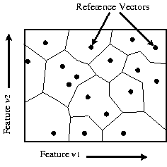
Figure 3. Classification using a Self-Organising Map. A tessellated feature space of two dimensions is formed by the proximal regions of a set of reference vectors. Each region corresponds to a distinct class (or subclass).

The task of learning is to position the reference vectors so that the tessellation they provide minimises the classification error. An input vector x is classified by finding the reference vector w_c that is the nearest-neighbour of x, as defined by the Euclidean metric:

.

The positioning of reference vectors effectively provides an estimate of the probability density function for each class. Positioning is achieved here using the optimised learning rate (OLVQ1) supervised learning algorithm. The algorithm simulates learning as a dynamic process that takes place over a number of discrete time slices (t_i). Initially, a number of reference vectors are introduced as {w_i(t): i = 1,..., N}. The class of each reference vector is calculated using the k-nearest neighbour method (MacQueen, 1967), then the positions of the reference vectors are updated according to the learning rules described below. Let x(t) be an input vector at discrete time t. The reference vector closest to x(t) is found using the above Euclidean distance equation. The reference vectors are then updated using the following rules:

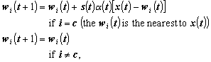
where s(t) takes the value +1 if the class of x(t) is the same as that of w_c(t) and -1 otherwise. The learning rate a (t) takes values between 0 and 1 and decreases over time. Individual reference vectors can have their own specific learning rate, set so that each training input vector affects the position of the reference vector with equal weight.

SOM and LVQ are chosen here since they are able to learn in a supervised and unsupervised mode, give fast convergence (around 18 sec on Pentium 233MHz machine for the experiments described here), have been shown to be good estimators of probability density functions (Kohonen, 1982) and can be organised into a hierarchy. Also, in contrast to many other forms of neural networks, they are remarkably simple to configure (e.g., Gahegan et al., 1999). The software used is available on the internet from http://www.cis.hut.fi/nnrc/index.html.

3. Experiments

3.1 The dataset used

The Kioloa Pathfinder Dataset is used for reporting purposes here, to facilitate direct comparison of classifier performance with previous work by the authors, colleagues and others using neural networks (Multi-Layer perceptron), decision trees and parametric classifiers on the same dataset (Lees and Ritman, 1991; Fitzgerald and Lees, 1994; Gahegan et al., 1999; German et al., 1997). This dataset contains a number of thematic environmental surfaces that can be grouped into dataspaces and has a well-documented set of groundcover samples with which the classifier can be trained and tested. Furthermore, the combined attribute space is complex, and defies a simplistic approach to classification. As Figure 1 shows, classes overlap, are poorly delineated, and do not always form a single cluster or region. Training samples have a large input vector (11 surfaces) and contain the full range of statistical types. The target domain is that of floristic classification, the differentiation of individual vegetation types (or vegetation niches), rather than the gross identification of urban, rural and water that are sometimes reported. Because of the large size of the input vector, the relatively small amount of training data (1,703 samples) and the non-uniqueness of class definitions, the dataset provides a good test of the learning and generalising capabilities of a classifier.

Provided in the dataset are the following themes: elevation (a DEM), geology (nominal data), surface water accumulation and flow length (simulated from the DEM), and several bands of Landsat Thematic Mapper (2, 4, 5, 7), aspect, slope and surface shape (calculated from the DEM).

3.2 Initial classification

To establish a benchmark for comparison, classification accuracy was first calculated by tackling the entire feature space together. Results obtained are shown below in Table 1 and show the percentage of examples classified correct for both the training and validation data.

Table 1: Initial results of classification using the entire feature space. Two thirds of all examples were used in training, with one third held over for validation. To examine the effects of different training, validation splits the data and were randomly reorganised 10 times to produce 10 distinct classifiers. The best result for both training and validation is shown in bold.

As is normally the case, the classifier performs less well on the unseen validation data. Nevertheless, a validation accuracy of around 62-66% on this dataset is a reasonable achievement given that traditional Maximum Likelihood returns an accuracy of about 40% on training. Notice that the performance is quite stable, to within 4%.

It is known that a SOM may develop poor mappings if elements of an input vector have different scales (Kohonen, 1995). This situation arises when an input vector consists of signals from different domains (Takatsuka, 1996), as is the case with this dataset. Standardising the dynamic range of each feature in the input vector ensures that any movements in a given direction in feature space are co-measurable. Table 2 shows the improvement encountered when the input data are scaled so that each dimension is normalised to have roughly the same standard deviation.

Table 2: More results using the entire feature space, but this time the input vector has each element scaled so that the dynamic range is standardised.

As expected, Table 2 shows a consistent improvement (of about 4%); however, examining the individual class accuracy reveals some serious difficulties in classifying certain landcover types. Table 3 gives a breakdown of results for a typical training run. Classes with fewer training examples (particularly classes 2 and 3) attract fewer reference vectors, hence, may be described poorly. As most neural classifiers, SOMs have an inductive bias towards classes with larger samples, since these large classes offer the greatest potential for gains in accuracy.

Table 3. A per-class assessment of classifier performance showing a large spread in accuracy due to problems of class separability and unequal numbers of training samples. Min Distance is the median of minimum distances, per class, among the reference vectors.

Note that there is a considerable spread in accuracy values, particularly at the validation stage. The overall result is largely determined by the classifier's performance on well-differentiable classes with large numbers of samples. Also, some landcover types achieve almost 100% accuracy, notably cleared land and water. The discrimination task for these classes is quite simple, whereas discrimination for most classes is problematic, as hinted at by the scatterplots shown in Figure 1. German et al. (1997) show how a study of the types of classification errors occurring can lead to insight into the complexity of the discrimination task.

To overcome this aspect of learning bias, it is necessary to have each class equally represented in the training sample. Where training data is in abundant supply, or can be gathered with ease, then overcoming this bias presents no real difficulty; however, this is not the case. One possibility is to reduce the number of samples to the lowest denominator (class 2) but this would involve discarding useful data. Another is to 'force' learning to occur on the difficult regions of the feature space by duplicating examples, effectively raising the number of samples to the highest denominator. This latter possibility was investigated, but, as might be expected, performance on generalisation was reduced. The classifier overtrains on the repeated identical examples for the under-represented classes. 

3.3 Classification using dataspaces

The experiments in this section use a feature vector that is partitioned into several dataspaces; thus, classification is a two-stage process as shown in Figure 2 (right side). Each dataspace is first classified or clustered in isolation, then the output from the dataspaces becomes the input for a final combination phase. In this manner, the overall classification task is reduced to a number of less complex sub-spaces.

The first experiment in this section uses an unsupervised SOM to effectively cluster regions of each dataspace, then LVQ is used to combine the outputs generated. The target classes are introduced into the training vector for LVQ, hence, it behaves as a supervised classifier. Results were obtained for different distinct splits of the feature vector into dataspaces. The results shown in Table 4 are for the following split: {dataspace 1 [North Aspect, East Aspect] dataspace 2 [elevation, slope, surface water accumulation, geology, surface shape] dataspace 3 [Landsat bands 2, 4, 5 and 7]}.

Table 4. A classification using dataspaces to initially cluster the data. In this particular example, accuracy on the training set is improved, but the improvement cannot be generalised to the unseen data.

Interestingly, performance on the training set improves, giving a higher average score and with even less variance (<2%). Validation shows that the classifier also outperforms the initial benchmark slightly (Table 1), but does not achieve the same level of performance as the second experiment using scaled input vectors.

There are a number of possible reasons why performance does not improve:

1. First, some over-training may have occurred, indicated by higher training scores and lower validation scores than in Table 2. Various different arrangements of neurons were tested for the dataspaces and these indicated that overtraining indeed could occur. An architecture of 10*10 neurons seemed to minimise the problem.
2. Second, input vectors are not scaled, so a performance penalty might be reasonably expected (as shown by the first two experiments). Interestingly, the arrangement of dataspaces that performed best was where dynamic ranges of variables were more consistent, and not where the strength of geographic theme was highest.
3. By choosing to form dataspaces where a high degree of structure and clustering is present, the task of discrimination may actually be made more difficult. Another possibility (to be investigated later) is to chose spaces that disperse the data as much as possible.
4. Finally, since clustering in the individual dataspaces is unsupervised then it is in no way directed towards the target of floristic classification. The clusters formed may relate poorly to the classification task, once it is introduced in the final section.

4. Conclusions

Some experiments are reported into the use of Self-Organising Maps and Learning Vector Quantisation as tools for geographic classification. From these experiments we make the following observations:

1. The classifiers appear to be stable. Without much effort in terms of experimental set-up and network architecture we were able to achieve results consistent to within about 4% across ten random splits of training and validation data.
2. Computationally, the technique is very undemanding--execution times are measured in seconds. Computational load compares favourably with backpropagation networks (which can take 10-30 minutes) and is similar to that of decision trees.
3. SOMs are particularly sensitive to differences in the dynamic range of the input variables. Better results follow when ranges are either co-measurable or normalised.
4. In terms of floristic classification, the classifier performs poorly where classes are poorly separable. While this might seem reasonable, performance could be bettered if decision rules were less hard (more probabilistic), allowing uncertainty to remain in the classification until the final stage. Tools that facilitate this approach (such as DONNET, German et al., 1997) are able to achieve about a 10% improvement in validation accuracy.

As with most neural techniques, the functioning of the classifier is difficult to explain in any language that is geographically meaningful. The outcome of training is a classifier whose decision rules are not known, the implicit domain structure is encoded in an arrangement of nodes (neurons) and their weighted inter-connections; thus, potentially useful insight into relationships within the data that may lend structure to the analysis will go unobserved.

4.1 Future Work

As is often the case when examining a new tool, there are more avenues to explore than can be covered in a single paper. Much remains to be tested, and the classifier still requires some 'packaging' in terms of configuration and ease of use. Future work will focus on the combination of both supervised and unsupervised approaches, and will aim to concentrate learning on the more problematic regions of the feature space. Dataspaces could be formed using standard measures of correlation or clustering such as the Mean Nearest Neighbour Distance (MNND), or possibly even the inverse of MNND, in an effort to provide a means for class discrimination. Finally, a more probabilistic version of the SOM is under development to pass on some measure of feature-space neighbourhood information to the LVQ supervised stage. 

References

Aspinall, R. J. and B.G. Lees, 1994. Sampling and Analysis of Spatial Environmental Data. Proc. 6th International Symposium on Spatial Data Handling, Ed: Waugh T C and Healey R G, Edinburgh, Scotland, pp. 1,086-1,098.

Bishop, C. M., 1995. Neural Networks for Pattern Recognition, Clarendon, New York, U.S.

Benediktsson, J. A., P.H. Swain and O.K. Ersoy, 1990. Neural network approaches versus statistical methods in classification of multisource remote sensing data. IEEE transactions on Geoscience and Remote Sensing, Vol. 28, No. 4, pp. 540-551.

Civco, D. L., 1993. Artificial neural networks for landcover classification and mapping. International Journal of Geographical Information Systems, Vol. 7, No. 2, pp. 173-186.

Dietterich, T. G., 1997. Machine learning research: four current directions. AI magazine, Winter 1997, pp. 97-136.

Fitzgerald, R.W. and B.G. Lees, 1994. Assessing the classification accuracy of multisource remote sensing data. Remote Sensing of the Environment, Vol. 47, pp. 362-368.

Freidl, M.A. and C.E. Brodley, 1997. Decision tree classification of land cover from remotely sensed data. International Journal of Remote Sensing, Vol. 61, No, 4, pp. 399-409.

Gahegan, M. and G. West, 1998. The classification of complex geographic datasets: an operational comparison of artificial neural network and decision tree classifiers, Proc. GeoComputation '9: 3^rd International Conference on GeoComputation, http://www.cs.curtin.edu.au/~mark/geocomp98/ geocom61.html.

Gahegan, M., G. German and G. West, 1999. Some solutions to neural network configuration problems for the classification of complex geographic datasets. Geographical Systems, [In press].

German, G., M. Gahegan and G. West, 1997. Predictive assessment of neural network classifiers for applications in GIS. Second International Conference on GeoComputation, Otago, New Zealand.

Hepner, G. F., T. Logan, N. Ritter and N. Bryant, 1990. Artificial neural network classification using a minimal training set: comparison to conventional supervised classification. Photogrammetric Engineering and Remote Sensing, Vol. 56, No. 5, pp. 469-473.

Kohohen, T., 1982. Self-organised formation of topographically correct feature map. Biological Cybernetics, Vol. 43, pp. 59-69.

Kohonen, T., 1995. Self-Organising Maps. Springer-Verlag, Berlin, Germany.

Lees, B. G. and K. Ritman, 1991. Decision tree and rule induction approach to integration of remotely sensed and GIS data in mapping vegetation in disturbed or hilly environments. Environmental Management, Vol. 15, pp. 823-831.

MacQueen, J., 1967. Some methods for classification and analysis of multivariate observations. Proc: 5^th Berkley Symposium, pp. 281-297.

Okabe, A., B. Boots and K. Sugihara, 1992. Spatial Tessellations: Concepts and Applications of Voronoi Diagrams. John Wiley & Sons, Chichester, England.

Paola, J.D. and R.A. Schowengerdt, 1995. A detailed comparison of backpropagation neural networks and maximum likelihood classifiers for urban landuse classification. IEEE transactions on Geoscience and Remote Sensing, Vol. 33, No. 4, pp. 981-996.

Takatsuka, M., 1996. Free-Form Three-Dimensional Object Recognition Using Artificial Neural Networks. Ph.D. thesis, Dept. of Electrical and Computer Systems Eng., Monash University, Clayton 3168 VIC, Australia.