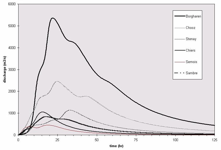
Figure 1: Flood hydrographs of several outlets in the Meuse catchment simulated using the PCRaster script. Water input to the model is a constant 5 cm layer of water in the entire catchment. Values do not represent reality.
A.P.J. De Roo
Joint Research Centre, Space Applications Institute,
AIS Unit Environment and Natural Hazards, TP 950, 21020 Ispra (Va), Italy
C.G. Wesseling & W.P.A. Van Deursen
PCRaster Environmental Software, P.O. Box 427, 3500 AK Utrecht,
The Netherlands
Although many GIS are very advanced in data processing and display, current GIS is not capable of physically-based modelling. Especially simulating transport of water and pollutants through landscapes is a problem in a GIS environment. A number of specific routing methods are needed in a GIS for hydrologic modelling, amongst those numerical solutions of the Saint-Venant equations, such as the kinematic wave approximation for transport of surface water in a landscape. The PCRaster Spatial Modelling language is a GIS capable of dynamic modelling. It has recently been extended with a kinematic wave approximation simulation tool to allow for physically based water flow modelling. The LISFLOOD model is an example of a physically-based model written using the PCRaster GIS environment. LISFLOOD simulates river discharge in a drainage basin as a function of spatial data on topography, soils and land cover. Although hydrologic modelling capabilities have largely increased, there is still a need for development of other routing methods, such a diffusion wave.
Keywords: Floods, GIS, PCRaster, LISFLOOD, hydrologic modelling, catchment, kinematic wave
Recently, dramatic flooding occurred in several regions of the world: Bangladesh (1988), Vaison La Romaine (France, 1992), Mississippi River (USA, 1993), Meuse (Netherlands, 1993), Piemonte (Italy, 1994), Rhine and Meuse (Netherlands, Belgium and Germany, 1995), Biescas (Spain, 1996), and the most recent floods of the Oder in The Czech Republic, Poland and Germany (1997). To assess the causes of these and other flood events, distributed hydrologic modelling at the scale of a large river basin is a very useful tool.
Physically-based modelling at the scale of an entire river basin requires large input databases. Therefore, a Geographical Information System is a very useful environment to model because of its advantages of data storage, display and maintenance (De Roo et al., 1989; Burrough and McDonnell, 1998). Thus, linking or integrating models with a GIS provides an ideal environment for modelling processes in a landscape. Three approaches exist for modelling within a GIS environment: loose coupling, tight coupling and embedded coupling (Wesseling et al. 1996). In loose coupling the GIS is used to pre-process the spatial data into the desired model input-file format, such as used by De Roo et al. (1989), De Roo (1996) and Kite et al. (1996). In tight coupling models and GIS, model input and output can be addressed directly by the GIS. In embedded coupling the model is written in an integrated programming language. The advantage of this is that the user can construct his or her own models as required. However, not many GIS are capable of physically-based modelling. Some GIS have some modelling capabilities, such as the AML language and the cell-based modelling tools of the Arc/Info GIS (such as the FlowAccumulation command) and the drain command in the Grass GIS. Using these tools, some transport modelling can be done.
At present, most GIS provides catchment analysis tools for delineation of catchments and definition of drainage networks. These tools, however, are not sufficient for dynamic modelling; they are not capable of solving transport operations through the defined network. Also, simulations in time are often not possible, such as simulating the catchment response to a rainfall timeseries. Ideally, for transport modelling one should be able to control the amount and velocity of water (or any other material) through the network: one would want to have 'access' to the algorithms describing this transport.
Therefore, there is a need for a GIS modelling environment that is capable of physically-based transport modelling. This paper describes such a GIS and as example the LISFLOOD river flooding model. An earlier example of embedded modelling is the LISEM catchment erosion model, which is described in De Roo et al. (1996).
The PCRaster spatial modelling language (Van Deursen, 1995; Wesseling et al. 1996) is an extension of the ideas behind Map Algebra and the Cartographic Modelling Language proposed by Berry and Tomlin (Berry 1987, Tomlin 1990) but includes ideas of iterations used in Dynamic Modelling and concepts for defining transport equations along the drainage network (in PCRaster referred to as Local Drain Direction network). Thus, PCRaster allows for developing physically-based transport models.
The syntax of the language is based on mathematical equations where each equation assigns the value of an expression to a single output. For example, an equation for sediment transport capacity of a water flow derived by Kirkby (1976)
G = C * Q^d * sin(S) * 10^-3
is applied to the raster maps CoverFactor (C), FlowVolume (Q) and Slope (S) with an exponent (d) of 1.7 using the command
TransportCapacity = CoverFactor*FlowVolume**1.7 *sin(Slope)*10E-3;
The command above is a point operation, where a new value for each location, a grid cell, is derived from different attribute values on that same location only. Global operators, where a new value for each location is derived from different attribute values on (possible) different locations, are also modelled as mathematical functions.
The set of available global operators in PCRaster is very extensive in comparison to the range of operations generally considered as Map Algebra. A rich suite of geomorphologic and hydrological operators is available. These include functions for hillslope and catchment analysis, and the definition of topology for modelling transport (drainage) of material over the local drain direction map with routing functions.
PCRaster is further illustrated by an example where a routing function (accuflux) is used to calculate the upstream area of one or more catchments. The operator accuflux calculates the accumulated amount of material that flows out of the cell into its neighbouring downstream cell. This accumulated amount is the material in the cell itself plus the amount of material in all upstream cells of the cell. The topological linkages defining upstream and downstream neighbours is given by a local drain direction map as the first argument. The second argument of accuflux is in general a map with material to be transported such as surface water as in the next example:
WaterFlow = accuflux(Ldd, WaterAmount);
Dynamic models are constructed by writing scripts containing series of statements (Van Deursen, 1995). The language has no explicit structures for iteration, although dynamic models do iterate in time. Instead, there are different sections that are controlled by the definition of a timer.
The timer section regulates the duration and time slice of the model through three parameters, starttime, endtime and timeslice.
The initial section sets the initial conditions for the model, including maps and non-spatial attributes. These values may be defined with one or more PCRaster operations. The dynamic section defines the operations for each time step that result in a map of values for that time step. Each time step consists of one or more PCRaster operations which are performed sequentially.
The next example shows a simplified model script that incorporates precipitation, infiltration and overland flow.
# <- this symbol is typed at the start of a comment line
timer
 1 28 1; # 28 timesteps of 6 hours

initial
 # coverage of meteorological stations for the whole area
 RainZones = spreadzone(RainStations,0,1);
 # create a map of infiltration capacity (mm/6hours),
 # based on a soilmap
 InfiltrationCapacity = lookupscalar(SoilInfiltrationTable,SoilType);

dynamic
 # add rainfall to surface water (mm/6hours)
 SurfaceWater = timeinputscalar(RainTimeSeries,RainZones);
 # compute both the runoff and actual infiltration
 Runoff, Infiltration =
  accuthresholdflux, accuthresholdstate(Ldd,SurfaceWater,InfiltrationCapacity);
 # output runoff at each timestep for selected locations
 report SampleTimeSeries = timeoutput(SamplePlaces, Runoff);
In this example, rainfall is the dynamic input. RainTimeSeries is a time table with the precipitation measured at several meteorological stations. RainZones does not represent the location of the stations but the area of pixels for which the measurement at that station is the best estimation of the actual precipitation at each pixel. Such a map can easily be computed from a station location map, as done in the initial section with the application of spreadzone. The RainZones map denotes for each pixel the column number in the time table. At each time step, timeinputscalar reads a row associated with the current time step and returns a map containing the column values as defined by RainZones. Note that the current time step is an implicit argument to all dynamic functions, such as timeinputscalar and timeoutput.
The second operation in the dynamic section transports the SurfaceWater over the local drain direction map Ldd. This is done with the accuthreshold operator which is one of the transport functions (named accu-operators) that accommodate transports restricted by certain transport functions. The accuthreshold operator transports water only once the infiltration capacity, given on the map InfiltrationCapacity, is exceeded. It results in two maps: a map with the actual infiltration (Infiltration) and a map with the amount of overland flow (Runoff). The map InfiltrationCapacity is calculated in the initial section on basis of a soil map (SoilType) and a cross table (SoilInfiltrationTable) that gives for each soil type the infiltration capacity.
The last statement of the example creates time series from certain locations in the Runoff map. These locations are identified by the SamplePlaces map. Each non zero value in the SamplePlaces map stands for a column in the time series (SampleTimeSeries). A PCRaster script that contains a dynamic section does not write any results to the database unless the keyword report is added. This prevents the surplus storage of intermediate results. Thus, typing the report before a statement like Runoff = accuthresholdflux(...) creates a stack of raster maps for each time step.
Other functions in the 'accu - family' include functions for limited transport capacity, or functions for transporting only a fraction of the input material. Experiments are carried out with travel-time approaches as well (Van Deursen, 1995).
The 'accu - approach' is not sufficient when the timestep of the model approaches the average traveltime through a cell, or whenever the number of pixels along the transport path is large. Due to the relatively simple schemes for solving the differential equations underlying this transport processes, in this case the PCRaster models become numerically very unstable. A more robust approach is needed. This approach can be found in the traditional algorithms for flood routing such as the kinematic wave approximation and the diffusion wave model (Chow et al. 1988; Fread 1993; Singh 1996). Recently, the kinematic wave has been implemented in PCRaster using the following syntax:
Q2 = kinematic(Ldd, Q1, q, ALPHA, beta, DTSEC,DX);
The new discharge Q2 at a certain location within the flow network (defined with Ldd) is calculated from the discharge Q1 from the previous time step at the same location and using Q2 from neighbouring upstream pixels. The kinematic wave can be used for hydrologic catchment models for overland flow routing of runoff and for channel routing under certain conditions. The kinematic wave cannot be used in case of backwater effects in rivers.
The following code gives an example of the use of the kinematic wave algorithm implemented in a PCRaster model script. The model script simulates water transport in a catchment with 1000 m pixels, using a 15 minute (900 seconds) timestep. These parameters are given in the 'binding' section of the script. Available water for transport is given in the initial map WH0. The Flow Network is defined in ldd.map, and slope GRADient is defined in slope.map. Several catchment outlets and sub-outlets are given in outlet.map. As stated in the 'timer' section, 500 time steps are simulated (125 hours).
In the dynamic section of the script the alpha variable is calculated first using cross section information (water depth and DX), Manning's n and slope gradient. In case of channels DX is replaced by the width of the channel. The next step is to calculate discharge. Subsequently the new discharge is calculated using the kinematic wave function. Then, the new water depth is derived from Q2 using the old alpha. This step is repeated to reduce numerical errors.
The results of the model are those that contain the 'report' statement. Flood hydrographs of several (sub-)outlets are presented in Figure 1. A map of gauging stations is presented in Figure 2. A map of overland flow and channel water depths is presented in Figure 3.
binding
 DTSEC=900;			# timestep (seconds)
 DX=1000;			# cell size (meters)
 beta=0.6;			# kinematic wave parameter: 0.6 is for broad sheet flow
 q=0.0;				# side-flow: not used
 WH0=whinit.map;		# initial wh.map (meters)
 GRAD=slope.map;		# slope map (-)
 Ldd=ldd.map;			# local drain direction map
 N=0.100;			# Manning's n
 OutFlowPoint=outlet.map;	# map with catchment outlets

timer
 1 500 1

initial
 WH=WH0;

dynamic
 ALPHA = (N*(DX+2*WH)**(2.0/3.0)/sqrt(GRAD))**beta ;
	# ALPHA is a roughness parameter in the kinematic wave formula;
	# WH is waterdepth (m), calculated using rainfall, interception and infiltration
 Q1 = if(ALPHA gt 0.0 , ((DX*WH)/ALPHA)**(1/beta) , 0.0);
	# Overland Flow Discharge, in m/s*m*m = m3/s
 Q2 = kinematic(Ldd, Q1, q, ALPHA, beta, DTSEC,DX);
	# Ldd is the Local Drainage Direction, the flowpath
 WH = ALPHA*(Q2**beta)/DX;
        # First approximation of new WH using old ALPHA (ok for small time steps)
	# WH is the flowdepth in m
 ALPHA = (N*(DX+2*WH)**(2.0/3.0)/sqrt(GRAD))**(beta);
 report WH = ALPHA*(Q2**beta)/DX;
        # Extra ALPHA calculation to calculate a more precise WH
 report Q2TSS=timeoutput(OutFlowPoint,Q2);
Figure 1: Flood hydrographs of several outlets in the Meuse catchment simulated using the PCRaster script. Water input to the model is a constant 5 cm layer of water in the entire catchment. Values do not represent reality.
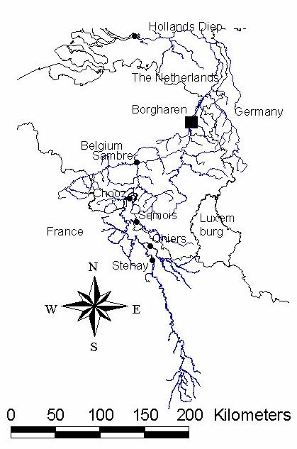
Figure 2: Selected discharge gauging stations in the Meuse catchment.
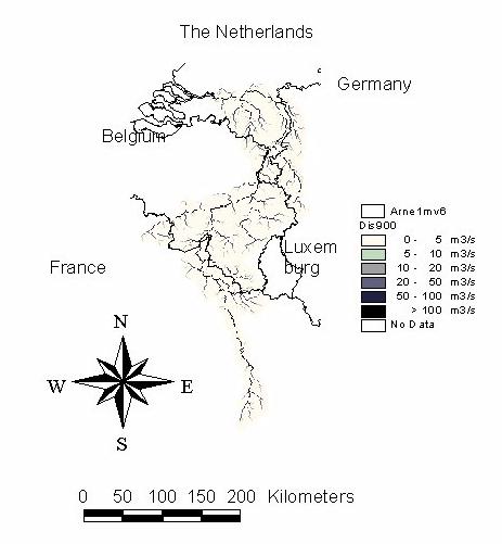
Figure 3: A map showing simulated water depths at time = 5 hours in the Meuse catchment, using the PCRaster script, from a 5 cm initial water layer input. Values range from 0-1 meter.
Using the kinematic wave function allows for a more robust method for solving transport equations. However, since backwater effects are not represented, other routing methods such as the diffusion wave need to implemented in the PCRaster GIS to further expand its capabilities for physically-based modelling.
To investigate the origin and causes of flooding and the influence of land use, soil characteristics and antecedent catchment saturation, the distributed catchment model LISFLOOD has been developed. LISFLOOD simulates runoff and flooding in large river basins as a consequence of extreme rainfall. LISFLOOD is a distributed rainfall-runoff model taking into account the influences of topography, precipitation amounts and intensities, antecedent soil moisture content, land use type and soil type.
The LISFLOOD model is built using the PCRaster Dynamic Modelling Language. Thus, the model uses square grids to represent the landscape. The grid size is user defined and the maximum number of grids is limited by computer memory only. Also, the simulation time step can be defined by the user. Processes simulated are precipitation, interception, snowmelt, evapotranspiration, infiltration, percolation, groundwater flow, lateral flow and surface runoff (Figure 4). For surface runoff and channel routing, a GIS-based kinematic wave routing module has been developed within PCRaster. Inundation extent will either be simulated by extrapolating predicted water levels onto a DEM, or LISFLOOD will be linked to an existing 2D or 3D model for detailed floodplain routing. Models built with the PCRaster Dynamic Modelling Language, such as LISFLOOD, have a very flexible model structure and are easy adaptable. The LISFLOOD model contains around 200 lines of code.
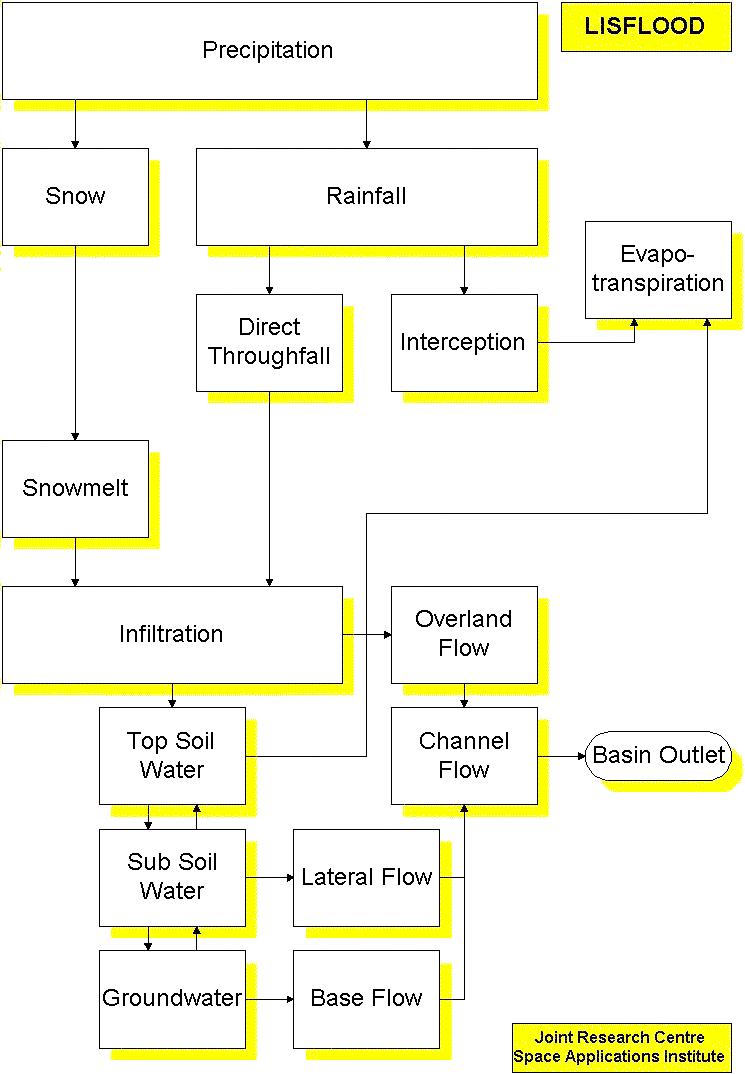
Figure 4: Flowchart of the LISFLOOD model.
LISFLOOD uses rainfall and temperature time series as input. Data from a large amount of meteorological stations can be used. At present, Thiessen polygons are used for interpolation, but other interpolation methods are examined. In order to account for orographic influences, spatial interpolation using a DEM is considered.
Infiltration is simulated using a two-layer Green-Ampt equation. Overland flow and channel flow are routed separately using the Manning equation and the kinematic wave approximation. For channel flow simulation, separate maps of the channel dimensions and Manning's n need to be provided.
Outputs of LISFLOOD are time series of discharge at user defined catchment outlets and sub-outlets. Furthermore, final maps of source areas of water (Figure 5), total rainfall, total interception, total infiltration etc. can be produced, as well as a series of maps showing changes in time of certain variables, such as the water depth in each pixel.
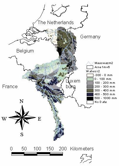
Figure 5: A map showing simulated source areas of water in the Meuse catchment, during the 1995 flood. Preliminary result, based on Belgian rain data only and using a preliminary version of LISFLOOD. Values shown are numbers of mm water contributing to the flood during a three month period. Negative values are net infiltrating areas.
In two pilot transnational European river basins the flooding problem is investigated using the LISFLOOD model: the Meuse catchment, covering parts of France, Belgium and The Netherlands, and the Oder basin, covering parts of The Czech Republic, Poland and Germany. The Meuse suffered from extreme flooding in December 1993 and January/February 1995. The Oder area was flooded in July 1997. In these catchments, LISFLOOD is tested, calibrated and validated before a detailed analysis of the causes of flooding can be examined.
At present, a 30-arc second digital elevation model is used as input, resulting in grids of 1000 by 1000 m. A 100 m DEM will be used for comparison in selected sub-catchments. The actual stream network is 'burned' into the DEM for better flow direction calculations. Slope gradient is also calculated, although interpretation of slope gradient at this scale is difficult.
Furthermore, hourly (Belgium, the Netherlands) and daily (France) rainfall of about 40 raingauges are used and interpolated using Thiessen polygons. Other methods are examined to include orographic influences, and to obtain a better spatial interpolation. Daily temperature data from European weather stations are taken from the MARS meteorological database available at JRC Ispra.
Soils information from the European Soils database (King et al. 1997) is used to obtain maps of soil depth and soil texture. Based on the HYPRES database (Lilly 1997, Wösten 1998) maps of saturated hydraulic conductivity and soil water content at saturation of topsoil and subsoil are constructed, based on average data for soil texture classes. In the near future, values will be based on individual soil mapping units.
The CORINE land use database of Europe is used to obtain maps of land use type. A difficult issue here is how to define and use the influence of land use on infiltration behaviour. Data in the HYPRES database, like many other soil physical measurements, are mostly carried out in vegetation free areas. There is a real lack of knowledge on the specific influence of vegetation on these soil physical properties. As for now in this study, a correction factor has been introduced for saturated hydraulic conductivity to account for vegetation influences based on limited literature data.
Information on soil cover by vegetation and leaf area index, used for interception and evapotranspiration calculations, are derived from satellite images..
In the Meuse pilot project, LISFLOOD is validated by streamflow data of gauging stations along the main river Meuse and data of several tributaries. These data are obtained from the National and Regional Water Authorities in the Netherlands, France and Belgium. SAR images will be used to validate the (maximum) extent of the flooded area in the floodplain.
The development, testing, calibration and validation is in full progress. First results are shown in Figure 5 showing source areas of water, and Figure 6, showing a preliminary comparison between measured and simulated discharge.

Figure 6: Measured and simulated discharge in the Meuse catchment during the flood of January and February 1995. Day 1 represents January 1 1995. Preliminary result based on Belgian rain data only and using a preliminary version of LISFLOOD.
No conclusions can be made from figure 6, since the model is in its early development. The timing of the flood seems to be reasonable, but the peaks and their shapes clearly need attention. But since percolation, subsurface flow and groundwater flow are not incorporated yet, and not all available rainfall data are used, a real assessment of the validity of the model cannot be made yet. In principle, the model should be able to provide predictions of flood inundation outside the period and circumstances under which it will be calibrated, but this is to be tested. In principle, the advantage of LISFLOOD over other, mostly lumped, models should be its possibility to evaluate spatial differences in soil and land use types. However, given the increased data need of the model this has still to be proven.
Embedded models in a GIS environment have many advantages over traditional loosely linked models and GIS. However, current GIS is lacking tools for developing physically-based models. Especially simulating transport of water and pollutants through landscapes is a problem in a GIS environment.
The PCRaster Spatial Modelling language is a GIS capable of dynamic modelling. Grid based models using input time series data such as changing rainfall amounts with time can be used, and output time series results such as discharge data can be produced. PCRaster contains several concepts for defining transport equations along the drainage network. It has recently been extended with a kinematic wave approximation simulation tool to allow for physically based water flow modelling. The LISFLOOD model is an example of a physically-based model written using the PCRaster GIS environment. LISFLOOD simulates river discharge in a drainage basin as a function of spatial data on topography, soils and land cover. LISFLOOD is currently being tested and validated in two transnational European catchments: the Meuse and the Oder catchment. Although hydrologic modelling capabilities have largely increased, there is still a need for development of other routing methods, such a diffusion wave, to allow simulating rivers with backwater effects.
Dr. Luca Montanarella (JRC Ispra), Christine Le Bas (INRA, Orleans) and Dr. Henk Wösten (Winand Staring Centre, Wageningen) are thanked for their help with the soils and HYPRES data. Stephen Peedell (JRC Ispra) is thanked for his valuable help on ArcInfo. Dr. Thierry Ubeda (JRC Ispra) is thanked for his help on getting the rainfall data with different formats in one file. Dr. Bart Parmet (RIZA, Arnhem) is thanked for providing GIS and discharge data on the Meuse catchment. Finally, Dr. Guido Schmuck is thanked for his contributions to the flood research at JRC.
Berry, J.K. 1987. 'Fundamental operations in computer-assisted map analysis', International Journal of Geographic Information Systems, 2, 119-136.
Burrough, P.A. and McDonnell, R.A. 1998. Principles of Geographical Information Systems. Oxford University Press. p. 333.
Chow, V.T, Maidment, D.R. and Mays, L.W. 1988. Applied Hydrology McGraw-Hill, p 572.
De Roo, A.P.J., L. Hazelhoff and P.A. Burrough 1989. 'Soil erosion modelling using 'ANSWERS' and Geographical Information Systems'. Earth Surface Processes and Landforms, 14, 517-532.
De Roo, A.P.J., C.G. Wesseling & C.J. Ritsema 1996. 'LISEM: a single event physically-based hydrologic and soil erosion model for drainage basins. I: Theory, input and output'. Hydrological Processes, 10-8, 1107-1117.
De Roo, A.P.J. 1996 'Soil Erosion Assessment Using GIS.' In: Singh, V.P. and Fiorentino, M. (eds.) Geographical Information Systems in Hydrology. Kluwer. 443 p.
Fread, D.L. 1993. 'Flow Routing'. Chapter 10 In: Maidment, D.R., Handbook of Hydrology. McGraw Hill, 10.1-10.36.
King, D., Daroussin, J., Jamagne, M., Le Bas, C. and Montanarella, L. 1997. The 1:1,000,000 soil geographical database of Europe. In: Bruand, A. et al. (eds.) The use of pedotransfer in soil hydrology research in Europe. INRA Orléans and EC/JRC Ispra.
Kirkby, M.J. 1976. 'Hydrological Slope Models: The Influence of Climate'. In: E. Derbyshire (Ed.), Geomorphology and Climate, John Wiley.
Kite, G.W., Ellehoj, E. and Dalton, A. 1996. 'GIS for Large-Scale Watershed Modelling'. In: Singh, V.P. and Fiorentino, M. (eds.) Geographical Information Systems in Hydrology. Kluwer. 443 p.
Lilly, A. 1997. A description of the HYPRES database (Hydraulic Properties of European Soils). In: Bruand, A. et al. (eds.) The use of pedotransfer in soil hydrology research in Europe. INRA Orléans and EC/JRC Ispra.
Singh, V.P. 1996. Kinematic Wave Modeling in Water Resources. John Wiley & Sons, 1399 p.
Tomlin, C.D. 1990. Geographic information systems and cartographic modelling. Prentice Hall, New York.
Van Deursen, W.P.A. 1995 'Geographical Information Systems and Dynamic Models: development and application of a prototype spatial modelling language. Netherlands Geographic Studies, 190. See also http://www.frw.ruu.nl/pcraster.html.
Wesseling, C.G., Karssenberg, D.J., Burrough, P.A. and Van Deursen, W.P.A. 1996. 'Integrated dynamic environmental models in GIS: The development of a Dynamic Modelling language. Transactions in GIS,1-1, 40-48.
Wösten, J.H.M. 1998 Personal Communication on HYPRES results.