Imports and Packages: Using JFreeChart
[Practical 7 of 11 - Part 1]
Storing Results:
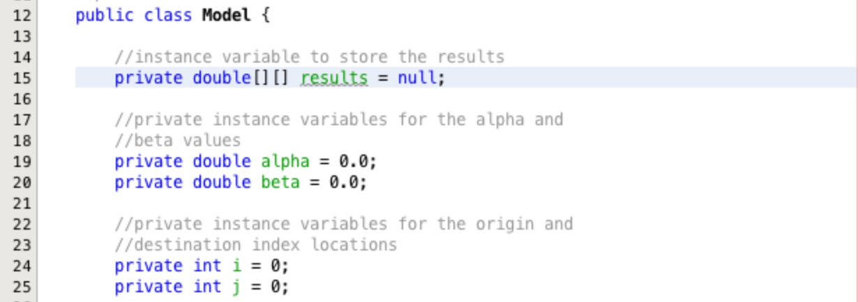
First we need to adapt our spatial interaction model code so that we store our results rather than printing them to the screen. Add a two dimensional double array instance variable to your Model class as shown in Figure 3.
Use the Refactor >>Encapsulate Fields... function to generate an accessor method to get the results, but do not supply one to set the results. We don't want to be able to set the results, only to calculate the results in the model.
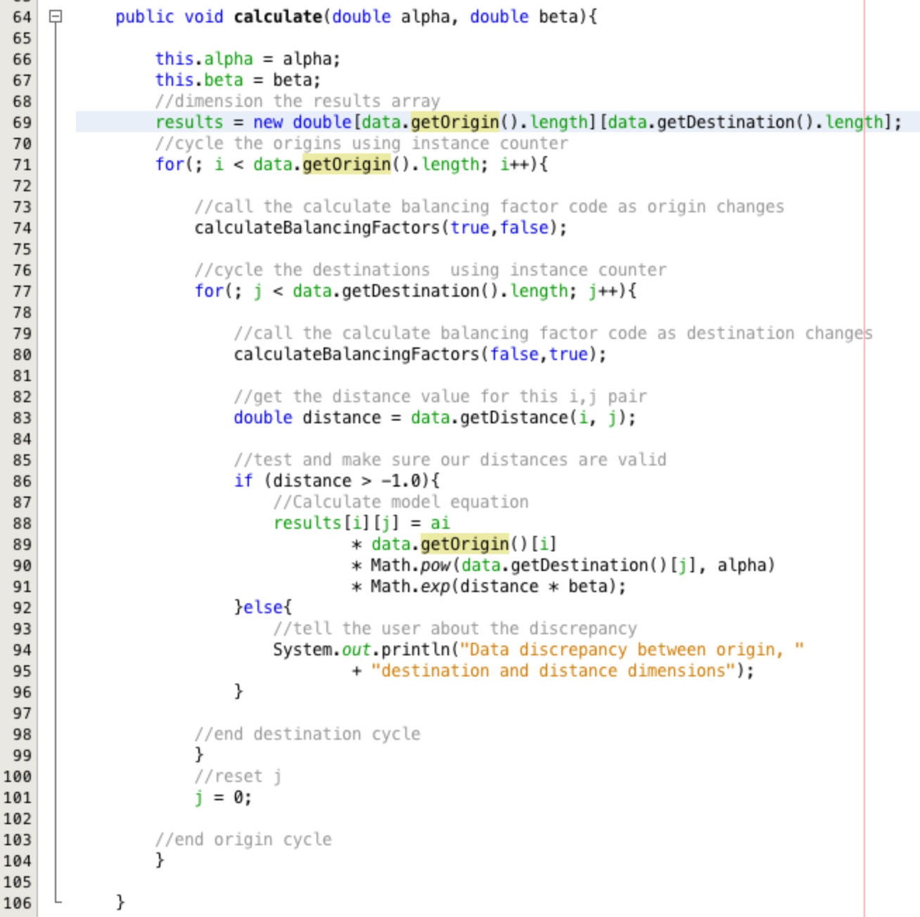
Now we need to remove all of the lines of code used to output the results to the screen and the associated comments.
There are four of these in the calculate method of the Model class. Remove the first
declaration of the output variable, String output = "";. The remaining places it has been used will be
highlighted by error lines. Delete all of these lines and the associated comments.
Now we can remove the declaration of the tij, double tij = 0.0;. Replace the assignment to the
tij variable when the equation is calculated with results[i][j]. This places the result of the
model equation straight into the result array in the corresponding origin / destination location.
The last change to the calculate method is to make sure that the results array is correctly dimensioned. At the top of the
calculate method add the line of code
results = new double[data.getOrigin().length][data.getDestination().length];. The calculate method should now look sinilar
Figure 4.
Getting Observed Data:
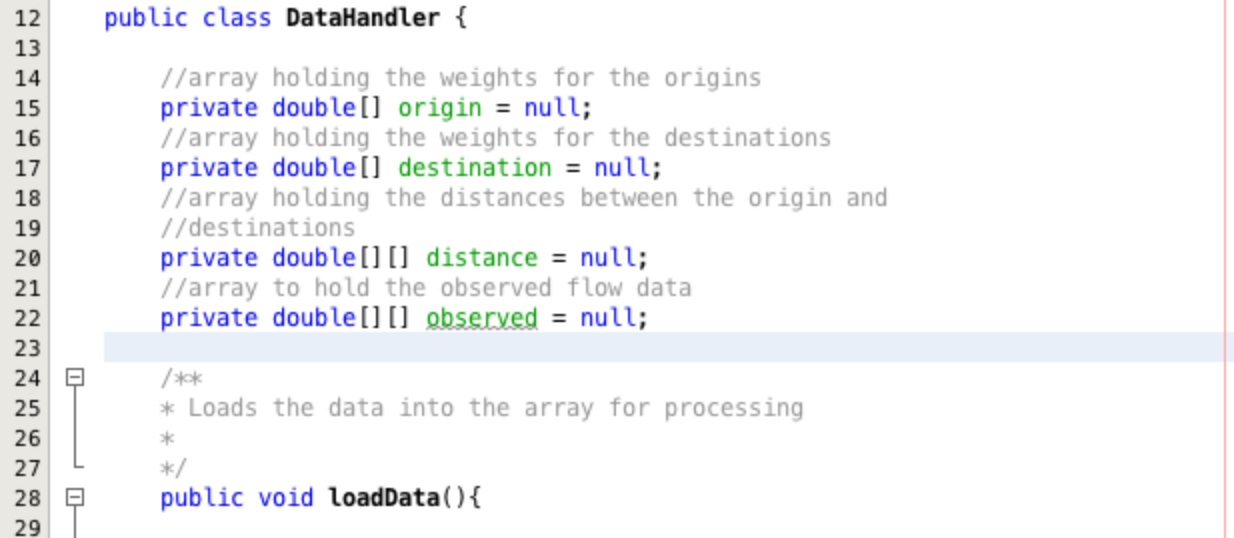
In the DataHandler class create a new two dimensional double array instance variable
called observed. Set it to equal null as shown in Figure 5.
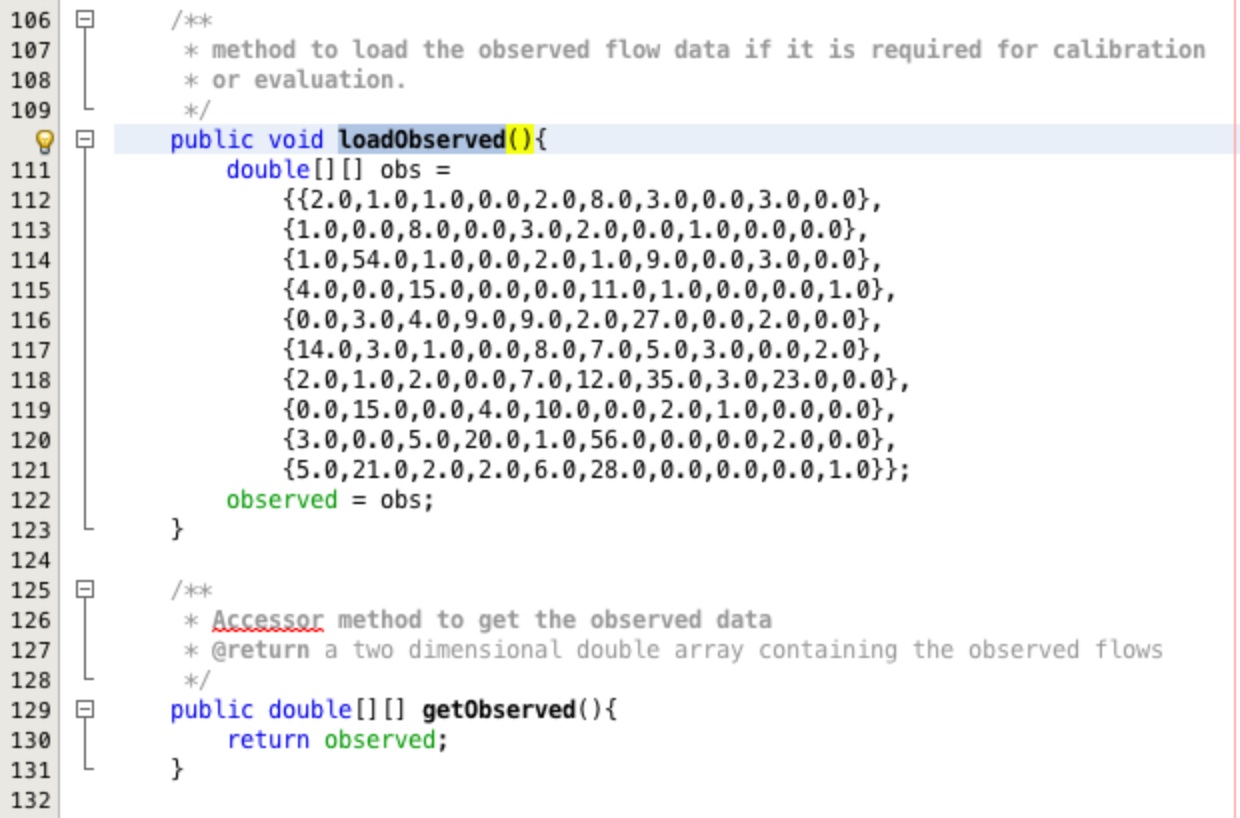
Add the two methods to load and access the data as shown in Figure 6. The code to populate the
loadObserved method is below.
double[][] obs =

            {{2.0,1.0,1.0,0.0,2.0,8.0,3.0,0.0,3.0,0.0},

            {1.0,0.0,8.0,0.0,3.0,2.0,0.0,1.0,0.0,0.0},

            {1.0,54.0,1.0,0.0,2.0,1.0,9.0,0.0,3.0,0.0},

            {4.0,0.0,15.0,0.0,0.0,11.0,1.0,0.0,0.0,1.0},

            {0.0,3.0,4.0,9.0,9.0,2.0,27.0,0.0,2.0,0.0},

            {14.0,3.0,1.0,0.0,8.0,7.0,5.0,3.0,0.0,2.0},

            {2.0,1.0,2.0,0.0,7.0,12.0,35.0,3.0,23.0,0.0},

            {0.0,15.0,0.0,4.0,10.0,0.0,2.0,1.0,0.0,0.0},

            {3.0,0.0,5.0,20.0,1.0,56.0,0.0,0.0,2.0,0.0},

            {5.0,21.0,2.0,2.0,6.0,28.0,0.0,0.0,0.0,1.0}};

        observed = obs;
Creating a Chart:
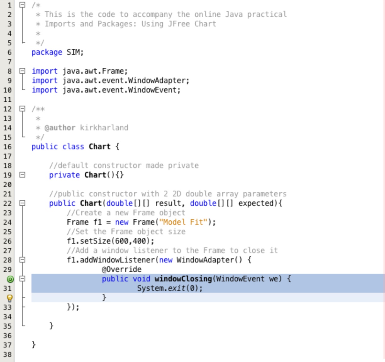
Create a new class in your SIM package called Chart. Create the default constructor as private
and add a constructor that accepts two two dimesional double arrays called result and
expected. Add the code to the constructor shown in Figure 7. When prompted add in the appropriate imports.
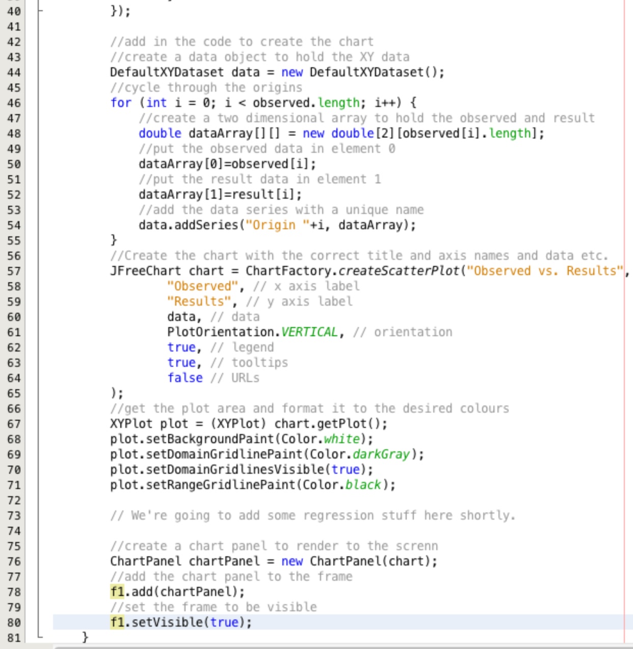
Now we'll add the graph. Add the code shown in Figure 8 to the constructor below the code to create the Frame, import the
appropriate packages as Netbeans prompts you to.
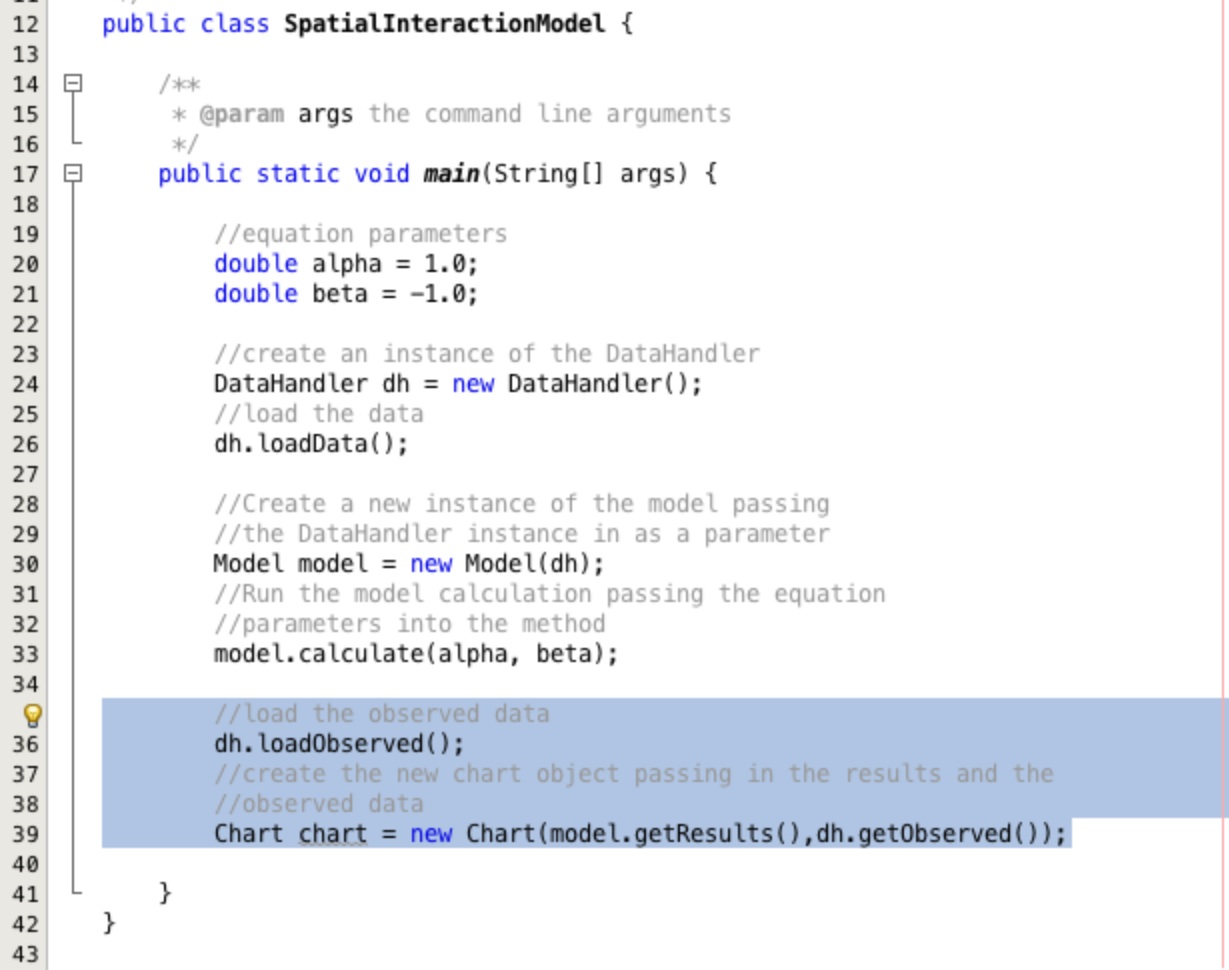
Drawing the Chart:
To get the chart to draw add the two lines of code highlighted in the Figure 9 to the SpatialInteractionModel
class.
Adding a Regression Line:
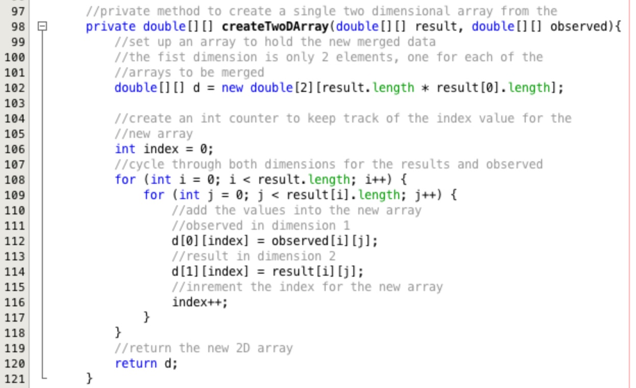
We are going to use all of the data points to create the regression line so we first need to turn
the two 2D arrays (observed and result) into one 2D array with a first dimension of 2. Each
corresponding origin-destination pair from both arrays should appear in the same index of the second dimension.
Add the code shown in Figure 10 to create a method to do this formatting. Study what the method is doing to manipulate the array. Can you see the assumptions it makes and some of the potential problems this may cause?
There are a wide variety of built in statistical functions in JFreeChart, you can find them in the
Docs under the
org.jfree.data.statistics package. Here we'll use the Regression.getOLSRegression() method.
Add the code highlighted in Figure 11 into the constructor of the Chart class below the comment
//We're going to add some regression stuff here shortly".
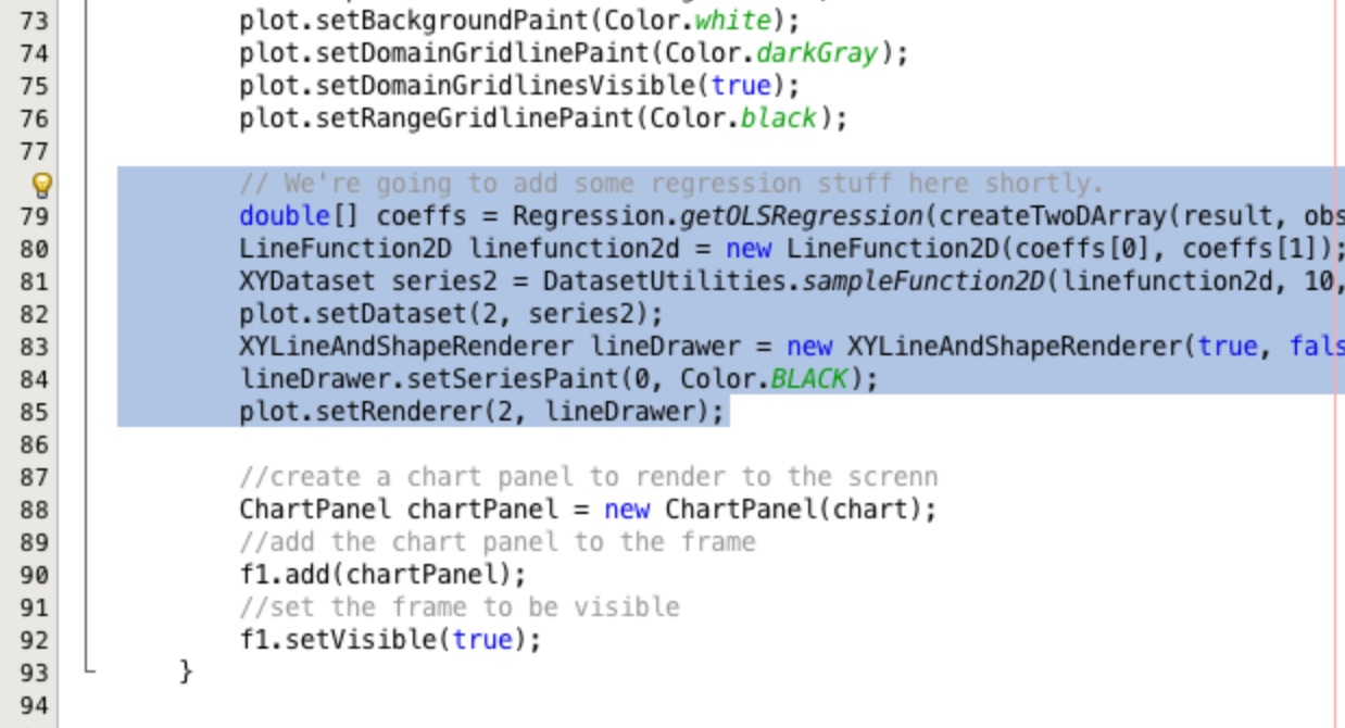
Have a careful look at the code we have used and compare it with the descriptions in the docs. The sampleFunction2D
method is useful - it generates a new point dataset based on a line equation. In this case the line equation is encapsulated
in linefunction2d which, in turn, is based on the intersect and gradient coefficients supplied by
getOLSRegression. The only problem is, we don't want another point dataset, we want a line, so when we add the
new data as the second series (setDataset(2, series2)) we also attach a renderer to it which isn't the default
point renderer.
Anyhow, run the code. Hopefully you'll see your original points with a regression line across them.
If you are interested in JFreeChart there's some more examples in the code cookbook, and the docs are useful, however your best source is the developer's guide - albeit it costs ~40 quid it is worth it, and includes all the source code for the examples on the JFreeChart website.
This practical has shown how we can import third party code to enhance our own work in a relatively painless way. We modified our model slightly to make it possible to store results and load observed data. This in turn made it possible to plot this data in a third party charting library.
This has been a relatively short practical and you may want to spend a little time reviewing the code used here to make sure you understand it or go back over some of the previous exercises to consolidate your knowledge.